Introduction
When researchers compare two laboratory instruments or diagnostic methods, it is common to collect repeated measurements from the same individual rather than only one observation. Traditional Bland–Altman analysis assumes that each subject contributes only one pair of observations. However, in many biomedical, clinical, pharmaceutical, and laboratory studies, multiple measurements are obtained from each participant.
Examples include:
- Blood glucose measured every hour
- Blood pressure measured repeatedly
- ECG recordings at different time points
- Multiple laboratory replicates
- Repeated analyzer measurements
Using the standard Bland–Altman method on repeated observations violates the assumption of independence. This can underestimate variability and produce misleading limits of agreement.
To solve this problem, MedCalc provides Bland-Altman Plot for Multiple Observations per Individual, which correctly accounts for repeated measurements from the same subject.
This tutorial explains the concept, assumptions, MedCalc options, practical example, result interpretation, and graph interpretation in detail.
What is a Bland-Altman Plot?
A Bland–Altman Plot is a graphical method used to evaluate the agreement between two quantitative measurement methods.
Instead of measuring correlation, it evaluates:
- Mean difference (bias)
- Random variation
- Limits of agreement
- Systematic error
The plot displays
X-axis
Average of both methods
Y-axis
Difference between methods
If the differences remain close to zero and lie within acceptable limits, the two methods may be considered interchangeable.
Why Use Multiple Observations per Individual?
Many experiments collect repeated observations from the same participant.
For example,
| Subject | Analyzer A | Analyzer B |
|---|---|---|
| Patient 1 | 112 | 114 |
| Patient 1 | 115 | 116 |
| Patient 1 | 118 | 120 |
| Patient 2 | 145 | 146 |
| Patient 2 | 147 | 149 |
Here,
Patient 1 contributes three measurements.
These observations are correlated.
Traditional Bland–Altman analysis assumes every observation is independent.
Therefore,
Standard Bland–Altman is not appropriate.
The repeated-measures Bland–Altman model adjusts for within-subject variability and between-subject variability.
Concept Behind the Analysis
The procedure estimates
- Mean bias
- Within-subject variation
- Between-subject variation
- Limits of agreement
- Confidence intervals
instead of treating every measurement pair as completely independent.
This provides more reliable estimates when repeated observations exist.
When Should This Method Be Used?
Use this analysis when
- Multiple measurements are collected per subject
- Two instruments measure the same variable
- Two laboratory analyzers are compared
- Clinical agreement is evaluated
- Repeated diagnostic measurements are available
When Should It NOT Be Used?
Do not use this method if
- Only one measurement exists per subject
- Data are categorical
- Variables are ordinal
- Measurements are from different individuals only
Data Structure Required in MedCalc
Example dataset
| Subject ID | Analyzer A | Analyzer B |
|---|---|---|
| 1 | 112 | 114 |
| 1 | 115 | 116 |
| 1 | 118 | 120 |
| 2 | 148 | 150 |
| 2 | 152 | 151 |
| 2 | 160 | 161 |
The Subject ID column identifies repeated observations.
📥 Download Example Data File
Step-by-Step Procedure in MedCalc
Step 1
Import your dataset into MedCalc.
Step 2
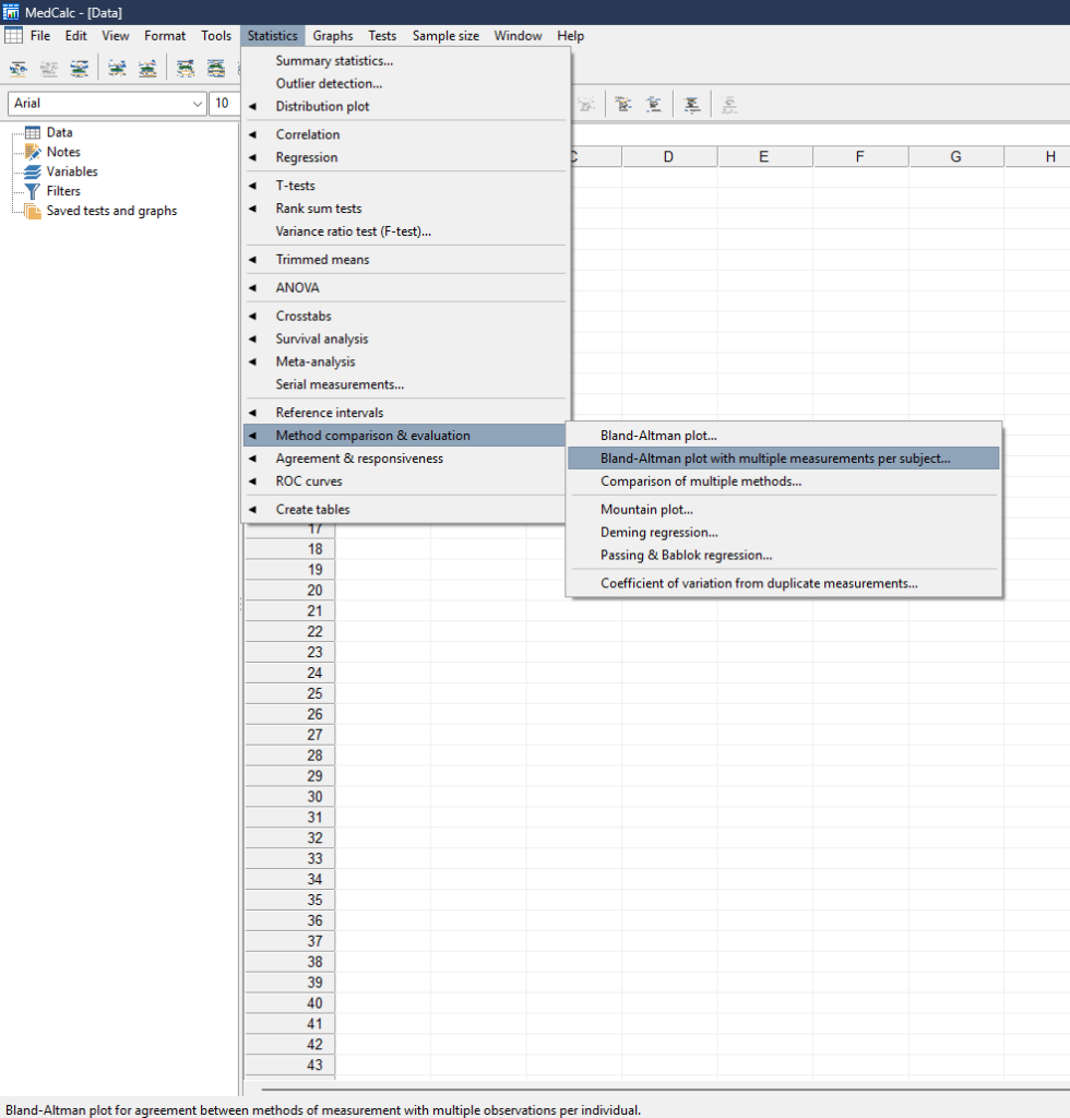
Click
Statistics → Method Comparison & Evaluation → Bland-Altman Plot with Multiple Measurements per Subject
Step 3
Select
First Method
Choose Analyzer A.
Step 4
Select
Second Method
Choose Analyzer B.
Step 5
Choose
Subject Identification
Select the Subject ID column.
Step 6
(Optional)
Choose a Filter variable if only certain observations should be analyzed.
Step 7
Choose the Model
✔ True value is constant in each subject
This assumes the actual value for each subject does not change during repeated measurements.

Step 8
Choose Plot Type
- Plot Differences ✔
- Plot Ratios
Differences are most commonly used.
Step 9
Choose X-axis
Options include:
- Mean of both methods
- First method
- Second method
- Geometric mean
- Sample rank
- Rank of first method
- Rank of second method
The default and most common choice is Mean of both methods.
Step 10
(Optional)
Specify
Maximum allowed difference between methods.
Step 11
Enable
✔ Draw line of equality (Difference = 0)
✔ 95% Confidence Interval of Limits of Agreement
Step 12
Click OK.
MedCalc will generate
- Statistical results
- Bland–Altman Plot
- Confidence intervals
- Limits of agreement
Explanation of Every MedCalc Option

First Method
The reference measurement.
Example
Analyzer A
Second Method
The new measurement technique.
Example
Analyzer B
Subject Identification
Required for repeated measurements.
It identifies which observations belong to the same subject.
Filter
Allows analyzing only selected observations.
True Value is Constant in Each Subject
Assumes the true value remains stable during repeated measurements.
Suitable for replicate laboratory analyses.
Plot Differences
Plots
Method A − Method B
Most frequently used.
Plot Ratios
Useful when proportional differences are expected instead of absolute differences.
Plot Against (X-axis)
Mean of both methods
Most commonly recommended.
First Method
Uses Method A values.
Second Method
Uses Method B values.
Geometric Mean
Useful for log-transformed data.
Sample Rank
Ranks observations instead of raw values.
Rank of First Method
Ranks Method A.
Rank of Second Method
Ranks Method B.
Maximum Allowed Difference
Defines acceptable clinical agreement.
Draw Line of Equality
Displays Difference = 0.
95% CI of Limits of Agreement
Shows uncertainty around upper and lower agreement limits.
Worked Example
Suppose
30 repeated observations are collected from multiple patients.
Two analyzers measure blood glucose.
Analyzer A
Existing laboratory instrument.
Analyzer B
New analyzer.
The goal is to determine whether both analyzers produce similar results.
MedCalc Results
From your uploaded output:
| Parameter | Value |
|---|---|
| Sample Size | 30 |
| Model | True value is constant in each subject |
| Plot Option | Plot differences |
| Mean Bias | -1.3333 |
| Lower Limit of Agreement | -13.0077 |
| 95% CI (Lower LOA) | -19.6798 to -10.6533 |
| Upper Limit of Agreement | 10.3411 |
| 95% CI (Upper LOA) | 7.9867 to 17.0131 |
Interpretation of the Results
Sample Size
Thirty paired observations were included in the agreement analysis.
Mean Bias
The average difference between Analyzer A and Analyzer B is -1.3333 mg/dL.
A negative bias indicates that Analyzer A tends to give slightly lower values than Analyzer B on average.
Limits of Agreement
The lower and upper limits of agreement are -13.0077 mg/dL and 10.3411 mg/dL, respectively. This means that approximately 95% of the differences between the two analyzers are expected to lie within this interval.
Confidence Intervals
The confidence intervals around the limits of agreement indicate the precision of these estimates. Narrower confidence intervals suggest more precise estimates of agreement.
Bland–Altman Plot Interpretation
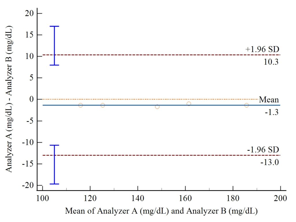
- A solid horizontal line representing the mean bias at -1.3333 mg/dL.
- Two dashed horizontal lines representing the 95% limits of agreement at approximately -13.0 mg/dL and 10.3 mg/dL.
- Most data points cluster close to the mean bias and fall well within the limits of agreement, with no obvious trend of increasing or decreasing differences across the measurement range.
Based on this plot, the two analyzers demonstrate good agreement, and there is no clear evidence of proportional bias over the observed concentration range. Whether the observed limits are clinically acceptable should be judged against the predefined allowable difference for the specific laboratory or clinical application.
Advantages
- Handles repeated observations correctly
- Produces reliable limits of agreement
- Accounts for within-subject correlation
- Ideal for laboratory validation studies
- Suitable for clinical method comparison
Limitations
- Requires repeated measurements
- Assumes correct subject identification
- Interpretation should include clinical acceptability, not just statistical agreement
- Extreme outliers can widen the limits of agreement
Conclusion
The Bland–Altman Plot for Multiple Observations per Individual in MedCalc is an essential method for assessing agreement between two quantitative measurement techniques when repeated measurements are obtained from the same subjects. By accounting for within-subject variability, it provides more accurate estimates of bias and limits of agreement than the traditional Bland–Altman approach. In your example, the analysis shows a small average negative bias (−1.3333 mg/dL) and 95% limits of agreement ranging from −13.0077 to 10.3411 mg/dL, with most observations falling within these limits, indicating generally good agreement between the two analyzers. Final acceptance should always be based on whether these differences are clinically acceptable for the intended use.