Introduction
Multiple regression analysis is a cornerstone of biostatistical research, enabling scientists to model and understand the relationship between one dependent variable and multiple independent variables. It allows for precise estimation of how each predictor contributes to the outcome while controlling for other variables.
In medical and biological research, MedCalc provides a user-friendly interface for performing multiple regression with extensive diagnostic and validation tools. This article provides a step-by-step explanation of multiple regression options in MedCalc, including methods (Enter, Forward, Backward, Stepwise), variable inclusion/removal thresholds, and residual tests.
The goal is to help researchers confidently use MedCalc’s regression features for clinical, epidemiological, and biological data interpretation.
What is Multiple Regression?
Multiple regression is an extension of simple linear regression that examines how two or more independent variables predict the value of a single continuous dependent variable.
The general equation is:
Y= b0 + b1X1 + b2X2 +…+ bnXn + e
Where:
- Y = Dependent variable (outcome)
- b₀ = Intercept (constant)
- b₁, b₂, … bₙ = Regression coefficients for predictors
- X₁, X₂, … Xₙ = Independent variables
- e = Error term
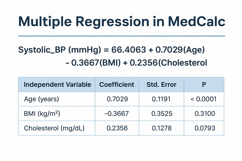
In medical contexts, for example, systolic blood pressure (Y) can be modeled as a function of age, BMI, and cholesterol levels (independent variables).
Performing Multiple Regression in MedCalc
When you open Multiple Regression in MedCalc (via Statistics → Regression → Multiple Regression), the dialog box presents several customizable options divided into different sections.
Below is a detailed explanation of each section.
1. Dependent and Independent Variables Section
In this section, you define your regression model structure.
- Dependent variable: The primary variable you want to predict or explain (e.g., Systolic_BP).
- Independent variables: Predictor variables that explain changes in the dependent variable (e.g., Age, BMI, Cholesterol).
You can include multiple predictors by selecting them from your dataset list.
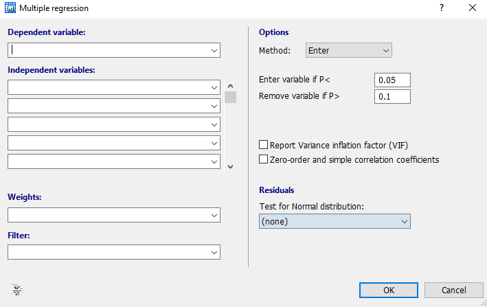
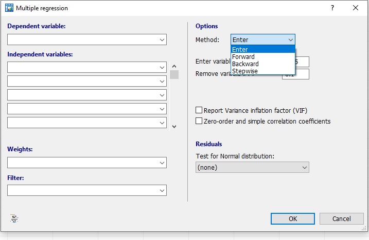
2. Method Options in MedCalc
MedCalc provides four main methods to enter variables into the regression equation. These are displayed under the “Method” dropdown list (see your first screenshot).
a. Enter Method
- All selected independent variables are entered into the model simultaneously.
- Use this method when theoretical justification exists for including all variables.
- Example: When analyzing the combined effect of Age, BMI, and Cholesterol on Systolic BP.
b. Forward Method
- Starts with no variables and adds them one by one.
- Each variable is included if it significantly improves the model (based on P < 0.05 or a chosen entry value).
- Best for exploratory analysis to identify key predictors.
c. Backward Method
- Starts with all selected variables.
- Removes variables stepwise that do not contribute significantly to the model (usually P > 0.1).
- Efficient when you suspect some predictors may not be important.
d. Stepwise Method
- A combination of forward and backward selection.
- Variables are added or removed based on significance criteria.
- Provides the most optimized model but should be used cautiously to avoid overfitting.
3. Entry and Removal Criteria
MedCalc allows you to specify criteria for variable inclusion or exclusion in stepwise or forward/backward methods.
- Enter variable if P < 0.05:
A variable is entered into the model if its probability of F (significance) is below this value.
Lower values (e.g., 0.01) make the inclusion more stringent. - Remove variable if P > 0.10:
A variable is excluded from the model if its probability of F exceeds this threshold.
A higher value retains more predictors; lower values yield a more parsimonious model.
4. Weights and Filter Options
These fields allow for additional control:
- Weights: Apply weights to data points if certain observations carry more importance (e.g., weighted least squares).
- Filter: Specify inclusion criteria (e.g., only include patients aged 40–60 years).
These options enhance model customization and ensure analysis relevance.
5. Residual Tests for Normal Distribution
Residual analysis checks whether the residuals (errors) from the regression follow a normal distribution, a key assumption of multiple regression.
MedCalc includes several tests under the Residuals section:
| Test Name | Purpose | Typical Use |
|---|---|---|
| Shapiro–Wilk Test | Most common and reliable test for normality | Small to medium sample sizes |
| Shapiro–Francia Test | Similar to Shapiro–Wilk but optimized for large samples | > 500 observations |
| D’Agostino–Pearson Test | Checks skewness and kurtosis | Medium to large samples |
| Kolmogorov–Smirnov Test | Compares residual distribution to normal curve | General-purpose |
| Chi-Squared Test | Categorical residual analysis | Less commonly used |
When normality is accepted (P > 0.05), regression assumptions are satisfied.
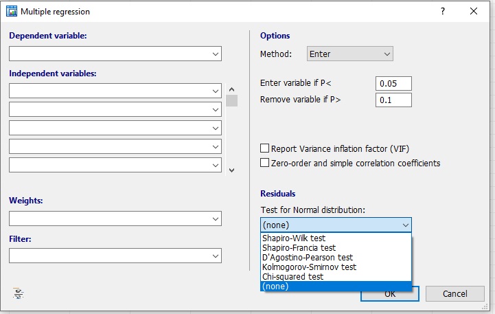
6. Variance Inflation Factor (VIF)
Selecting the “Report Variance Inflation Factor (VIF)” checkbox enables the calculation of multicollinearity among predictors.
- VIF > 10 indicates a high correlation between predictors, suggesting redundancy or overlapping information.
- High multicollinearity can distort regression coefficients and weaken interpretation.
This diagnostic helps ensure the reliability of your regression model.
7. Zero-Order and Simple Correlation Coefficients
Enabling this checkbox displays the correlation between each independent variable and the dependent variable.
It helps visualize how strongly each predictor is linearly associated before adjusting for others.
For example:
- Age vs. Systolic BP = r = 0.9988
- BMI vs. Systolic BP = r = 0.9804
These values indicate strong positive associations.
Example Table: Interpretation of Regression Output
| Predictor | Coefficient (b) | Std. Error | P-value | Interpretation |
|---|---|---|---|---|
| Age (years) | 0.7029 | 0.1191 | < 0.0001 | Significant positive effect on blood pressure |
| BMI (kg/m²) | -0.3667 | 0.3525 | 0.3100 | No significant effect |
| Cholesterol (mg/dL) | 0.2356 | 0.1278 | 0.0793 | Borderline significance |
8. Analysis of Variance (ANOVA) Table in MedCalc
The ANOVA section in MedCalc provides:
- F-ratio = 3569.8
- P < 0.0001
This indicates that the regression model as a whole is statistically significant.
It confirms that at least one of the independent variables significantly predicts the dependent variable.
9. Checking Model Assumptions
Before final interpretation:
- Confirm residuals are normally distributed (Shapiro–Wilk P > 0.05).
- Check for linearity and absence of multicollinearity (VIF).
- Ensure independence of errors and homoscedasticity.
These steps validate the reliability of your model.
10. Practical Applications in Biostatistics
- Predicting disease risk based on biomarkers.
- Assessing how multiple physiological parameters affect blood pressure or glucose.
- Estimating the impact of age, BMI, and cholesterol on cardiovascular risk.
MedCalc simplifies such analyses by providing immediate significance levels, confidence intervals, and diagnostics.
Conclusion
Multiple regression in MedCalc offers an efficient way to model complex biomedical relationships with precision. The software’s method options (Enter, Forward, Backward, Stepwise), residual tests, and VIF reporting make it a versatile tool for biostatistical research.
By understanding each option in the regression dialog box, users can select appropriate methods, verify assumptions, and interpret results accurately.
Ultimately, mastering these tools empowers researchers to translate quantitative data into meaningful biological insights.