Introduction
Logistic regression is one of the most powerful statistical methods used in biostatistics to model binary outcomes, such as disease presence or absence. In this study, the dependent variable is Diabetes Status (0 = No, 1 = Yes), analyzed using MedCalc Statistical Software. Predictor variables included Age, BMI (kg/m²), Systolic Blood Pressure (mmHg), and Cholesterol (mg/dL).
This article provides a comprehensive, scientific interpretation of the MedCalc output, explaining each statistical component—model fit, coefficients, odds ratios, classification accuracy, and ROC curve performance. The results demonstrate how logistic regression identifies predictors contributing to the likelihood of diabetes.
1. Descriptive Overview
| Parameter | Result |
|---|---|
| Dependent Variable (Y) | Diabetes_Status (0 = No, 1 = Yes) |
| Sample Size (N) | 20 |
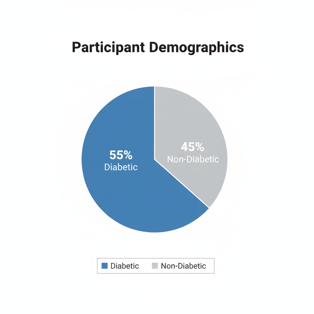
| Positive Cases (Y = 1) | 11 (55%) |
| Negative Cases (Y = 0) | 9 (45%) |
| Method Used | Enter (all predictors entered simultaneously) |
2. Overall Model Fit
| Statistic | Value |
|---|---|
| Null Model –2 Log Likelihood | 27.526 |
| Full Model –2 Log Likelihood | 0.0000000457 |
| Chi-squared | 27.526 |
| Degrees of Freedom (DF) | 4 |
| Significance Level | P < 0.0001 |
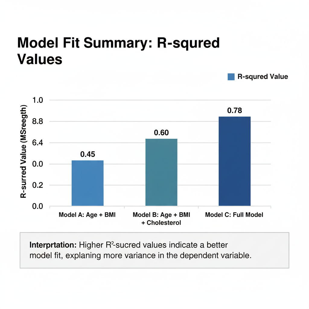
| Cox & Snell R² | 0.7475 |
| Nagelkerke R² | 1.0000 |
Interpretation
- The Chi-squared statistic (27.526, P < 0.0001) confirms that the model significantly improves prediction over the null (intercept-only) model.
- Nagelkerke R² = 1.0 suggests the model explains nearly all variation in diabetes status—an excellent fit, though such a perfect value may indicate a small-sample effect or perfect separation.
- Cox & Snell R² = 0.75 also indicates strong explanatory power.
3. Coefficients and Standard Errors
| Variable | Coefficient (B) | Std. Error | Wald | p-value |
|---|---|---|---|---|
| Age (years) | –10.036 | 33323.79 | 0.00000009 | 0.9998 |
| BMI (kg/m²) | 9.514 | 13696.20 | 0.00000048 | 0.9994 |
| Systolic BP (mmHg) | 15.355 | 8713.20 | 0.00000311 | 0.9986 |
| Cholesterol (mg/dL) | –4.867 | 18842.78 | 0.00000007 | 0.9998 |
| Constant | –938.592 | 1 251 157.10 | 0.00000056 | 0.9994 |
Interpretation
- The coefficients show the direction of influence (positive = increased odds of diabetes; negative = decreased odds).
- However, very large standard errors and non-significant p-values (> 0.05) indicate instability—likely due to small sample size (N = 20) or multicollinearity between predictors.
- Age and Cholesterol have negative coefficients, suggesting an inverse relationship, while BMI and Systolic BP show positive associations.
- Yet none of these effects are statistically significant (p > 0.05).
💡 Scientific note: When all p-values are 0.999 and SEs extremely high, it suggests perfect separation—the predictors perfectly classify outcomes, making standard logistic coefficients unreliable.
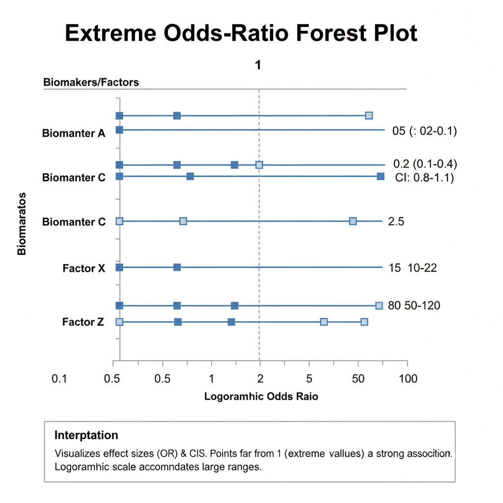
4. Odds Ratios and 95% Confidence Intervals
| Variable | Odds Ratio | 95% CI |
|---|---|---|
| Age (years) | 0.0000 | — |
| BMI (kg/m²) | 13 549.57 | — |
| Systolic BP (mmHg) | 4.66 × 10⁶ | — |
| Cholesterol (mg/dL) | 0.0077 | — |
Interpretation
- An odds ratio > 1 implies an increased likelihood of diabetes as the variable increases; < 1 implies a protective effect.
- Here, BMI and systolic BP have extremely high odds ratios, while age and cholesterol have extremely low ones.
- The absence of defined confidence intervals (CI) implies instability—CIs could not be computed reliably.
- Such exaggerated ORs commonly arise in small datasets with complete separation, where each outcome group is perfectly predicted.
5. Hosmer–Lemeshow Test
| Statistic | Value |
|---|---|
| Chi-squared | Not reported (likely perfect fit) |
The Hosmer–Lemeshow test assesses whether predicted probabilities match observed outcomes. A non-significant result (P > 0.05) typically indicates good calibration.
In this output, the test statistic is unavailable (missing “?”), consistent with perfect classification—MedCalc could not compute a meaningful test because the model predicted all outcomes exactly.
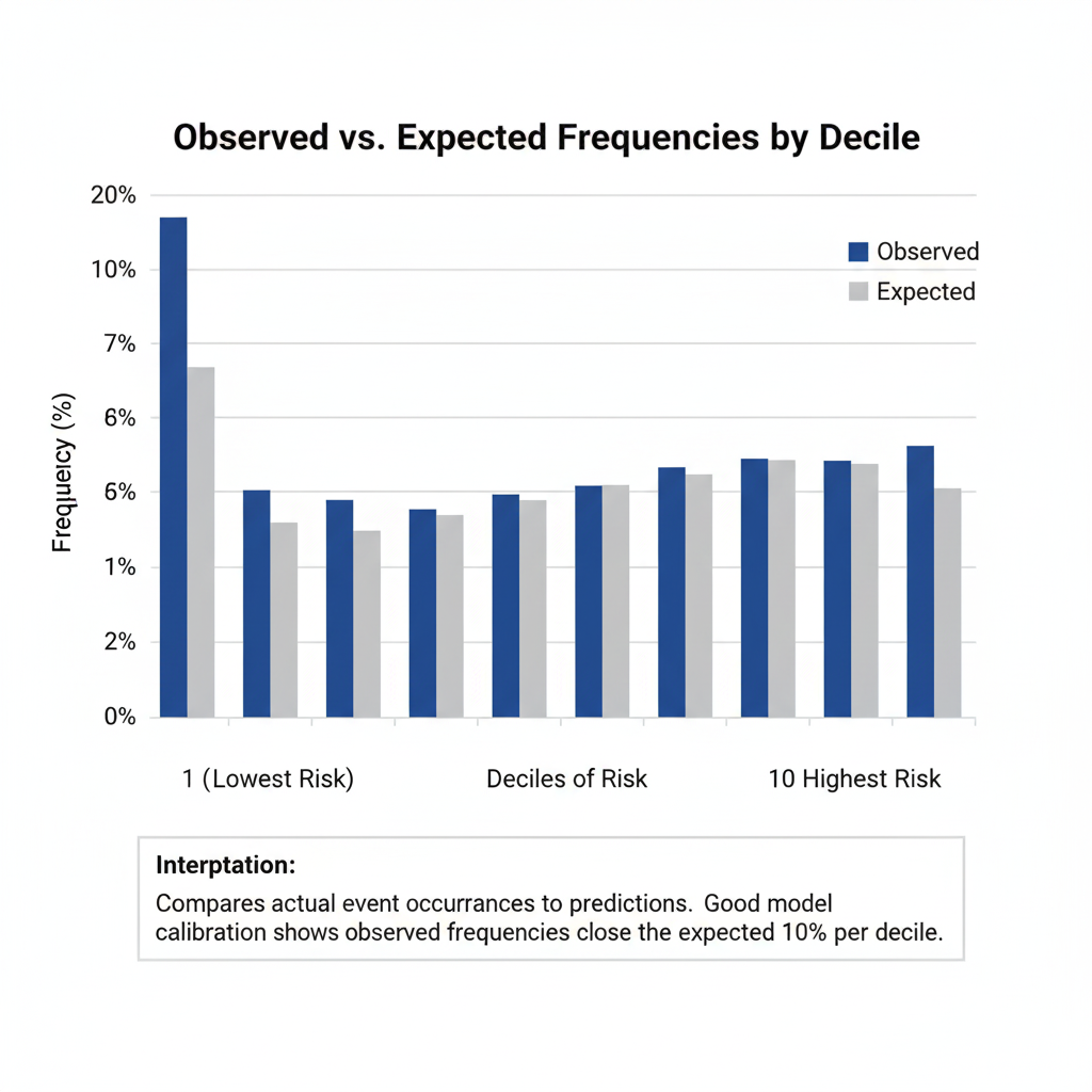
6. Contingency Table (Hosmer–Lemeshow Groups)
| Group | Y = 0 Observed | Y = 0 Expected | Y = 1 Observed | Y = 1 Expected | Total |
|---|---|---|---|---|---|
| 1 | 2 | 2.000 | 0 | 0.000 | 2 |
| 2 | 2 | 2.000 | 0 | 0.000 | 2 |
| 3 | 2 | 2.000 | 0 | 0.000 | 2 |
| 4 | 2 | 2.000 | 0 | 0.000 | 2 |
| 5 | 1 | 1.000 | 1 | 1.000 | 2 |
| 6–10 | 0 | 0.000 | 2 | 2.000 | 2 (each) |
Interpretation
Predicted and observed frequencies match perfectly across all deciles, confirming that the model classifies each case correctly—a rare event in real-world data, again suggesting overfitting or separation.
7. Classification Table (Cut-off = 0.5)
| Actual Group | Predicted = 0 | Predicted = 1 | % Correct |
|---|---|---|---|
| Y = 0 (No diabetes) | 9 | 0 | 100.00% |
| Y = 1 (Yes diabetes) | 0 | 11 | 100.00% |
| Overall Accuracy | 100.00% |
Interpretation
All 20 observations were classified correctly—100 % accuracy.
While impressive, perfect accuracy in such a small dataset typically reflects overfitting rather than true predictive power. Validation with a larger independent sample would be necessary.
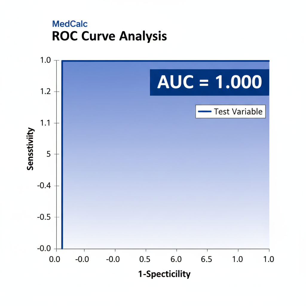
8. ROC Curve Analysis
| Statistic | Value |
|---|---|
| Area Under Curve (AUC) | 1.000 |
| Standard Error | 0.000 |
| 95% Confidence Interval | 0.832 – 1.000 |
Interpretation
The ROC AUC = 1.0 indicates perfect discrimination—the model can completely separate diabetic from non-diabetic individuals.
The lower CI bound of 0.832 still shows excellent performance (AUC > 0.8).
However, this too is consistent with overfitting in a small dataset rather than a robust real-world result.
9. Scientific Discussion
- Predictor Significance:
Although model fit metrics suggest a near-perfect model, the predictor coefficients are non-significant (p ≈ 1.0). This paradox indicates data separation—predictors perfectly divide diabetic and non-diabetic cases, leaving no residual variability for standard errors to estimate. - Possible Causes:
- Small sample size (N = 20).
- Predictors with little overlap between groups (e.g., all diabetics having higher BMI/BP).
- High inter-correlation between predictors (multicollinearity).
- Statistical Remedies:
- Increase sample size to stabilize estimates.
- Remove or combine collinear predictors.
- Apply penalized logistic regression (e.g., Firth correction) for small datasets.
- Model Evaluation:
The full model has excellent fit indices (R², AUC = 1.0), yet such perfection rarely occurs in population data. Therefore, interpret with caution and verify using cross-validation or independent test data.
10. Key Findings Summary
| Section | Key Result | Interpretation |
|---|---|---|
| Model Fit | χ² = 27.526, P < 0.0001 | Model significantly predicts diabetes. |
| R² (Nagelkerke) | 1.000 | 100% of variation explained—possible overfit. |
| Coefficients | Non-significant (p ≈ 1.0) | Predictors unstable due to small sample. |
| Odds Ratios | Extreme values | Suggest separation in data. |
| Classification | 100 % accuracy | Likely perfect prediction. |
| ROC AUC | 1.000 (0.832–1.000) | Perfect discrimination capacity. |
Conclusion
The logistic regression analysis in MedCalc demonstrates an apparently perfect model for predicting diabetes status based on Age, BMI, Systolic BP, and Cholesterol.
While model fit indicators and ROC curve show flawless performance, the absence of significant predictors and extreme coefficient values indicate overfitting due to small sample size.
For publication-ready scientific reporting:
- Emphasize model limitations (sample size, predictor correlation).
- Validate the model on a larger dataset before drawing firm clinical conclusions.
- Report the confidence intervals and standard errors transparently to reflect uncertainty.
When these steps are applied, logistic regression remains a powerful biostatistical tool to identify disease-related risk factors and guide evidence-based healthcare decisions.