Introduction
In biomedical and pharmaceutical research, the relationship between a drug dose and its biological response is often nonlinear. While linear regression provides a straight-line relationship between variables, it may fail to capture the curvature present in real-world data. Quadratic (Second-Degree Polynomial Regression) is an extension of linear regression that incorporates a squared term, allowing the model to describe curved relationships between independent (predictor) and dependent (response) variables.
In this tutorial, we use MedCalc Statistical Software to analyze the relationship between Drug Dose (mg) and Enzyme Activity (U/L) using a second-degree polynomial regression model. This example demonstrates how to perform the analysis, interpret the coefficients, assess model fit, and examine residuals.
Watch the Video Tutorial
🎥 Watch the complete step-by-step guide on YouTube below:
What is Quadratic Regression?
Quadratic regression models are used when data points form a parabolic (curved) pattern rather than a straight line. The model has the form:
y=a+bx+cx2
where:
- y = dependent variable (response)
- x = independent variable (predictor)
- a = intercept
- b = linear coefficient (slope of the line)
- c = quadratic coefficient (curvature)
A negative quadratic coefficient indicates a concave-down curve (an inverted U-shape), while a positive coefficient represents a concave-up pattern.
Data Description
The dataset consists of 25 observations of drug doses (in mg) and corresponding enzyme activity levels (U/L). The analysis was carried out in MedCalc
| Variable | Description | Units |
|---|---|---|
| Drug Dose | Independent variable (X) | mg |
| Enzyme Activity | Dependent variable (Y) | U/L |
| Sample Size | n = 25 | — |
Model Summary and Equation
From MedCalc output, the quadratic regression equation is:
y = 15.0604 + 1.5278x – 0.01073x2
This model indicates that:
- The intercept (15.06) represents the estimated enzyme activity when drug dose = 0 mg.
- The linear term (1.5278) shows that initially, enzyme activity increases with drug dose.
- The negative quadratic term (-0.01073) implies that after reaching a certain point, enzyme activity starts to decrease with higher doses, forming a concave-down parabola.
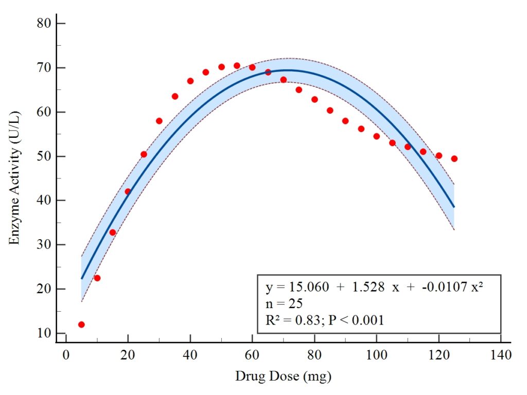
This image visually represents how enzyme activity increases to a maximum and then declines, illustrating the nonlinear response to increasing drug dose.
Statistical Summary from MedCalc
| Parameter | Value | Interpretation |
|---|---|---|
| Sample size (n) | 25 | Number of observations used |
| R² (Coefficient of determination) | 0.8331 | 83.31% of variation in enzyme activity is explained by drug dose |
| Residual standard deviation | 6.3628 | Indicates the average deviation of observed values from predicted values |
| F-ratio | 54.9171 | Measures overall model significance |
| Significance level | P < 0.0001 | Model is highly significant |
Interpretation:
The R² = 0.83 suggests that the model explains a substantial proportion of the variance in enzyme activity. The F-statistic (54.9) with P < 0.0001 confirms that the regression model is statistically significant — meaning the quadratic relationship between drug dose and enzyme activity is not due to random chance.
Analysis of Variance (ANOVA) Table
| Source | DF | Sum of Squares | Mean Square | F-Ratio | P-Value |
|---|---|---|---|---|---|
| Regression | 2 | 4446.71 | 2223.35 | 54.92 | <0.0001 |
| Residual | 22 | 890.68 | 40.49 | — | — |
| Total | 24 | 5337.39 | — | — | — |
Interpretation:
- The regression model explains most of the total variation in enzyme activity (4446.71 out of 5337.39).
- The F-ratio (54.9) indicates that the model provides a significantly better fit than a model without predictors.
Residual Analysis
Residuals represent the difference between observed and predicted values. Analyzing them helps confirm model validity.
| Test | Statistic | P-Value | Interpretation |
|---|---|---|---|
| Shapiro–Wilk | W = 0.9534 | P = 0.2990 | Residuals follow a normal distribution |
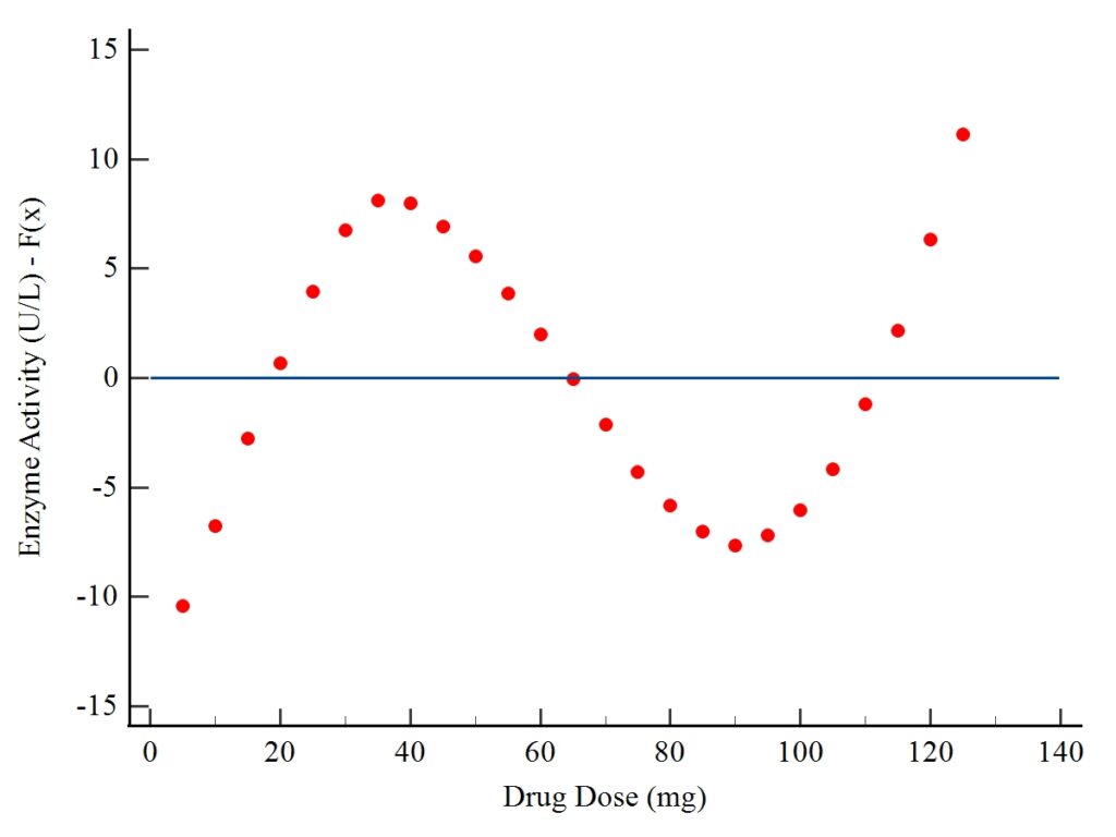
Interpretation of Residual Plot:
The residuals oscillate around the horizontal zero line, suggesting no systematic deviation from the fitted model. The normality test (P = 0.299) confirms that residuals are normally distributed — validating model assumptions. However, a mild cyclical pattern suggests possible higher-order curvature not fully captured by the quadratic model, but the overall fit remains strong.
Interpretation of Coefficients
| Coefficient | Symbol | Estimate | Interpretation |
|---|---|---|---|
| Intercept | a | 15.0604 | Baseline enzyme activity when dose = 0 mg |
| Linear | b | 1.5278 | Initial increase of enzyme activity per mg of drug dose |
| Quadratic | c | -0.01073 | Rate at which enzyme activity decreases after the peak dose |
The negative quadratic coefficient (-0.01073) implies that enzyme activity follows a parabolic path — increasing at low doses, peaking at a certain optimal level, then declining at higher doses. This pattern is biologically plausible, as excessive doses may inhibit enzyme function or cause feedback suppression.
Finding the Optimal Drug Dose
The vertex (maximum point) of a quadratic equation y = a + bx + cx2 occurs at:
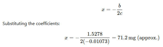
Thus, the optimal drug dose for maximum enzyme activity is around 71 mg. Beyond this dose, enzyme activity begins to decline.
Predicted Maximum Enzyme Activity
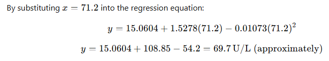
Hence, maximum predicted enzyme activity ≈ 70 U/L at a dose of 71 mg.
Biological and Clinical Interpretation
This result reflects a dose-response curve, a common feature in pharmacological studies. Initially, increasing the drug dose enhances enzyme activity due to substrate availability or activation of metabolic pathways. However, at higher concentrations, enzyme activity decreases — possibly due to saturation effects, feedback inhibition, or toxic responses.
The quadratic model effectively captures this biological phenomenon, providing an optimal dosage range for experimental or therapeutic consideration.
Model Validation and Goodness of Fit
Several aspects confirm that the quadratic model is valid:
- High R² (0.83) indicates good predictive power.
- Residuals are normally distributed (P = 0.299).
- Significant F-test (P < 0.0001) confirms model relevance.
- Visual inspection of residual plot shows no major outliers or heteroscedasticity.
Thus, the quadratic regression model provides a statistically sound and biologically meaningful explanation of the data.
Advantages of Using MedCalc for Polynomial Regression
MedCalc provides an intuitive interface for performing quadratic regression, making it ideal for researchers in biomedical sciences. Key advantages include:
- Automatic computation of R², F-tests, and ANOVA tables.
- Residual plots and normality tests for model validation.
- Graphical display of fitted curve with confidence bands.
- Exportable results for publication or reporting.
- Simple model specification using “Second-Degree Polynomial Regression” under the Regression module.
Summary of Regression Output (From MedCalc)
| Statistical Indicator | Value | Interpretation |
|---|---|---|
| Regression Equation | y = 15.0604 + 1.5278x – 0.01073x² | Best-fit model |
| R² | 0.8331 | Strong model fit |
| F-Ratio | 54.9171 | Model is significant |
| P-Value | < 0.0001 | Highly significant |
| Residual SD | 6.3628 | Moderate dispersion |
| Normality (W) | 0.9534 (P=0.299) | Accept normality |
When to Use Quadratic Regression in Biostatistics
Quadratic regression is appropriate when:
- The scatter plot shows a curved (nonlinear) pattern.
- There is an initial increase followed by a decrease in the response variable.
- Biological mechanisms suggest an optimal or threshold effect.
Common examples:
- Dose-response relationships
- Growth curves
- Enzyme kinetics
- Environmental tolerance ranges
Conclusion
This analysis demonstrates how Quadratic (Second-Degree Polynomial) Regression can model complex, curved relationships in biological data. Using MedCalc, we established that enzyme activity depends nonlinearly on drug dose, with an optimal value of approximately 71 mg, achieving ~70 U/L enzyme activity. The model fit was strong (R² = 0.83, P < 0.001), and residuals met the normality assumption.
Quadratic regression thus serves as a vital tool for exploring nonlinear relationships in biostatistics, pharmacology, and environmental sciences. Its ease of implementation in MedCalc makes it particularly accessible to students and researchers who require statistically rigorous yet user-friendly analytical methods.