Introduction
In the world of data science, not all relationships are straight lines. Real-world phenomena—from biological growth rates to market trends—often bend, accelerate, or level off in ways that simple linear regression cannot fully capture. When a linear model fails to describe such non-linear relationships, polynomial regression becomes an essential extension.
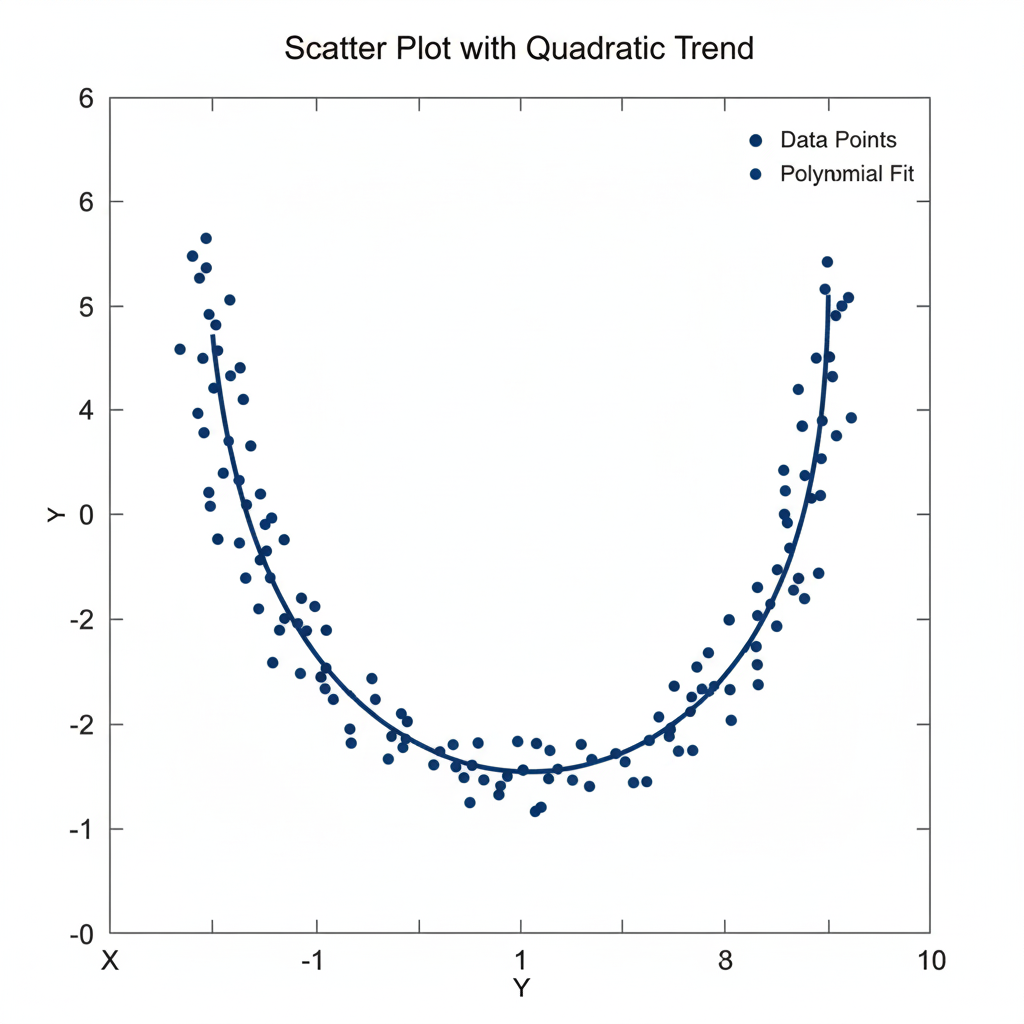
A second-degree polynomial regression model—commonly called a quadratic model—adds a squared term of the predictor variable to model a single curve or “bend” in the data. Its equation takes the form:
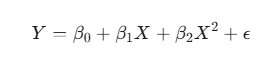
Here, Y is the dependent variable, X the independent variable, and the coefficients (β0,β1,β2) describe the curve’s position and shape.
This article dives into the essentials of the second-degree polynomial regression model—its mathematical foundation, practical implementation, interpretation, and common pitfalls such as overfitting and multicollinearity. Whether you’re a biostatistician, data analyst, or student, mastering this model can help you uncover meaningful patterns hidden within your curved data.
Understanding the Math Behind the Curve
The term polynomial regression may sound complex, but the concept is straightforward. It’s an extension of linear regression where the model includes powers of the independent variable. The reason it’s still considered linear lies in the coefficients—it remains linear in the parameters (β), not in the predictor variable X.
The Second-Degree Equation Explained
The general form is:
Let’s break it down:
- Y: The dependent or target variable (e.g., yield, weight, enzyme activity).
- X: The independent or predictor variable.
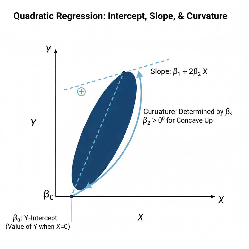
- β0: The intercept — the value of YYY when X=0X = 0X=0.
- β1: The linear effect of XXX on YYY.
- β2: The quadratic effect, determining the curvature of the line.
- ε: The random error term, representing unexplained variation.
Even though the model produces a parabolic curve, it is solved using the same Ordinary Least Squares (OLS) technique as linear regression because the coefficients enter the equation linearly.
Solving for the Coefficients: The Least Squares Approach
The goal of OLS is to find coefficient estimates that minimize the sum of squared residuals (SSR) — the squared difference between observed and predicted values.
In practice, this involves using matrix algebra to solve for the coefficient vector β:
β=(XTX)−1XTY
This allows us to compute the best-fitting curve through the data points, balancing the linear and quadratic effects.
Implementing Quadratic Regression in Practice
Now that we understand the math, let’s move to the practical side — implementing quadratic regression in software like Python or R.
Step-by-Step Implementation Guide
1. Data Preparation
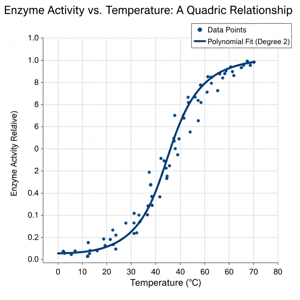
Begin by plotting a scatter plot to identify if the data shows curvature. If the pattern appears non-linear (e.g., U-shaped or inverted-U), a quadratic model is appropriate.
2. Feature Transformation
Add a new variable representing the square of X:
| X | X² | Y |
|---|---|---|
| 1 | 1 | 2.3 |
| 2 | 4 | 3.5 |
| 3 | 9 | 6.1 |
| 4 | 16 | 8.9 |
Here, X2 allows the model to bend to fit the data trend.
Example transformation:
If X=[1,2,3], then transformed features become:
[[1,1],[2,4],[3,9]]
3. Model Fitting
In Python (scikit-learn):
from sklearn.linear_model import LinearRegression
from sklearn.preprocessing import PolynomialFeatures
import numpy as np

X = np.array([1, 2, 3, 4, 5]).reshape(-1,1)
Y = np.array([2.3, 3.5, 6.1, 8.9, 12.0])

poly = PolynomialFeatures(degree=2)
X_poly = poly.fit_transform(X)
model = LinearRegression().fit(X_poly, Y)
In R:
model <- lm(Y ~ X + I(X^2), data = dataset)
summary(model)
4. Prediction and Visualization
After fitting the model, generate predictions and overlay the fitted quadratic curve on your scatter plot.
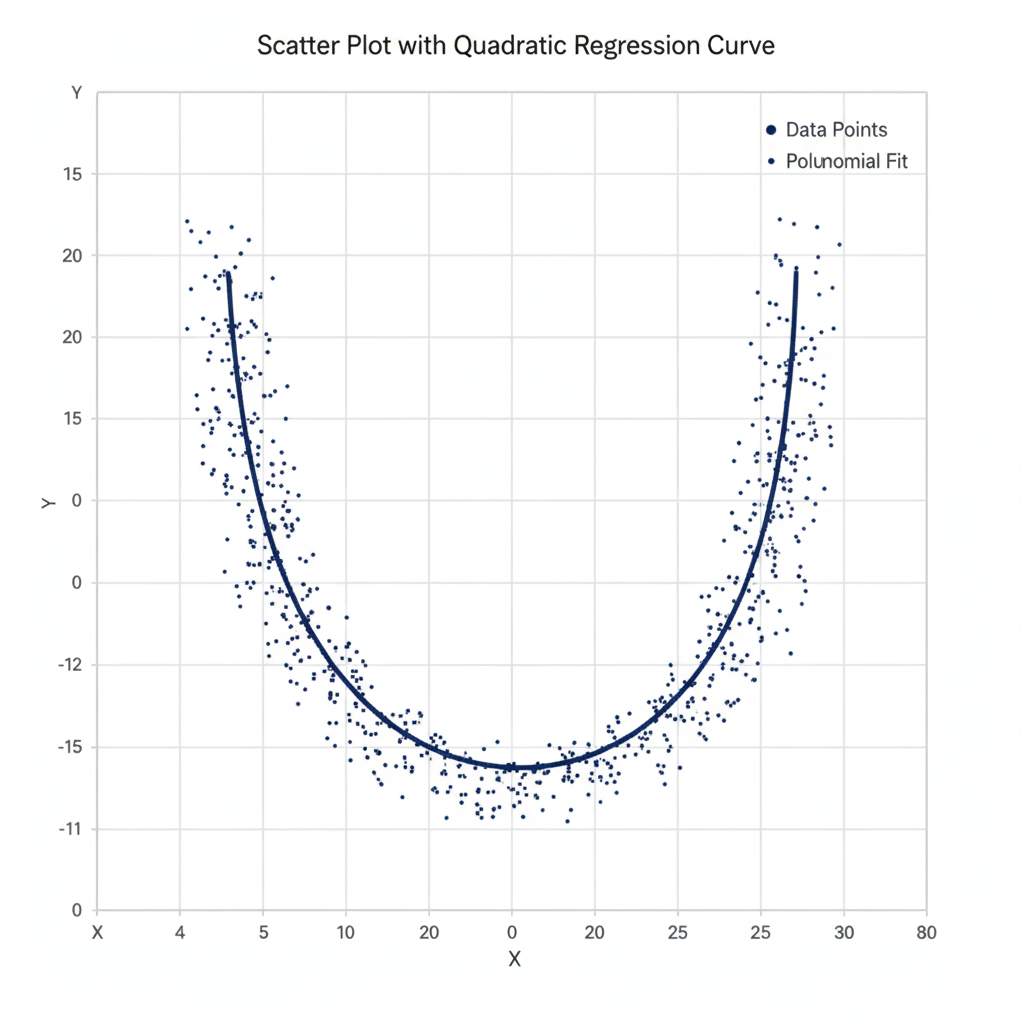
Table 1: Key Libraries and Functions for Implementation
| Language | Feature Transformation | Model Fitting | Evaluation |
|---|---|---|---|
| Python | PolynomialFeatures(degree=2) | LinearRegression() | r2_score() |
| R | I(x^2) in formula | lm() | summary() |
Interpreting the Model’s Results
Understanding the model’s output is essential for meaningful interpretation.
The Meaning of the Coefficients
- β0 (Intercept): The expected value of Y when X=0.
- β1 (Linear term): Represents the linear rate of change when X is small.
- β2 (Quadratic term): Determines the curvature — whether the parabola opens upward (β2>0) or downward (β2<0).
Unlike linear regression, here the slope is not constant. The rate of change of YYY with respect to XXX changes continuously according to:
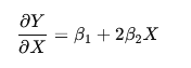
This means that for each unit increase in X, the slope itself shifts, controlled by β2.
Analogy:
Imagine a car. In linear regression, the car drives at a constant speed. In quadratic regression, the car accelerates or decelerates — the rate of change itself changes as you move along X.
Model Evaluation Metrics
To assess how well the model fits the data:
| Metric | Description |
|---|---|
| R² | Proportion of variance in YYY explained by XXX and X2X^2X2. |
| Adjusted R² | Penalizes unnecessary variables — checks if X2X^2X2 truly improves the model. |
| p-values | Test the significance of coefficients. |
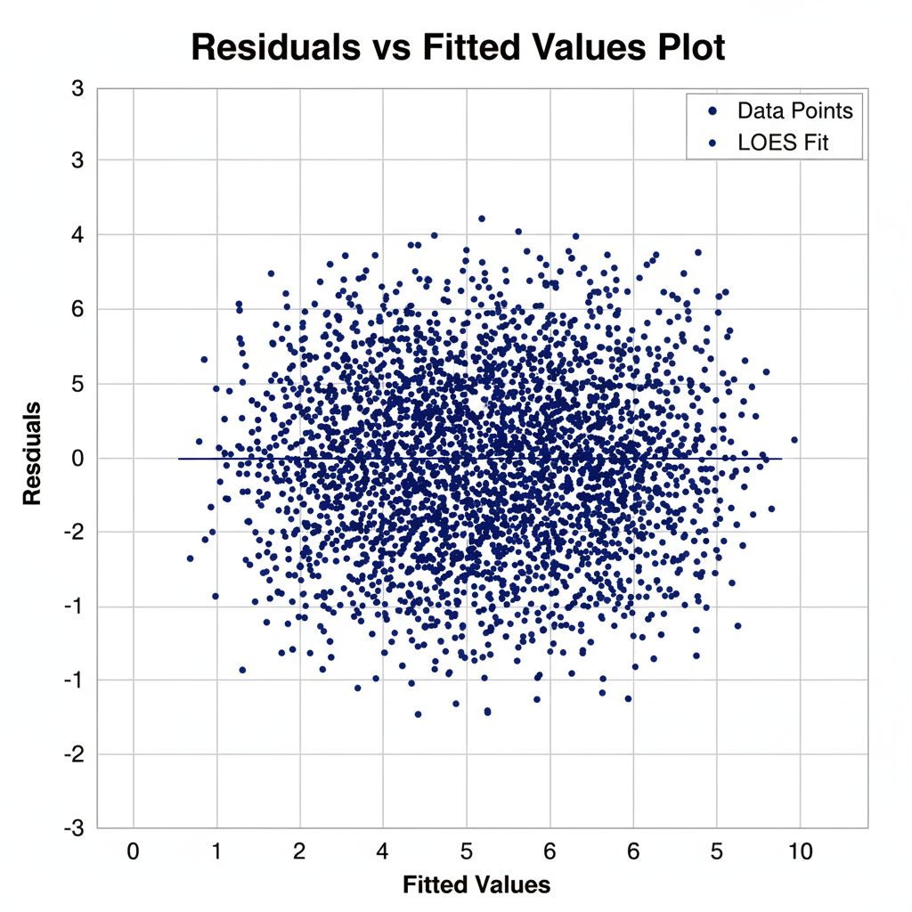
| Residual Analysis | Ensures that residuals are randomly distributed. |
Common Pitfalls — Overfitting and Multicollinearity
Polynomial regression adds flexibility, but it also introduces risks.
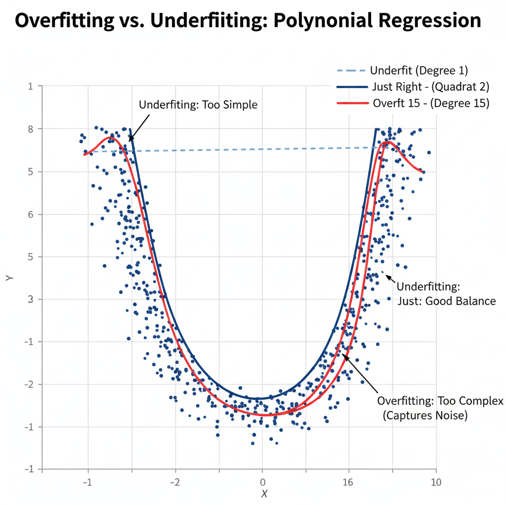
Overfitting — The Main Danger
While a second-degree polynomial (quadratic) is generally safe, higher-degree models can overfit, meaning they capture noise instead of genuine patterns. Overfitting results in poor generalization to new data.
Solution:
Use cross-validation to find the optimal degree of polynomial that balances bias and variance. Always visualize residuals and avoid unnecessary model complexity.
Multicollinearity
A subtle issue arises because X and X2 are often highly correlated. This can inflate standard errors, making coefficients unstable and harder to interpret.
Solution:
Center the variable before squaring it. That is, replace X with:
Xcentered = X −mean(X)
Then compute X2centered. This reduces multicollinearity without changing the overall fit.
Example (in R):
dataset$X_centered <- dataset$X - mean(dataset$X)
model <- lm(Y ~ X_centered + I(X_centered^2), data = dataset)
This simple transformation can dramatically improve model stability and interpretability.
Conclusion
The second-degree polynomial regression model is one of the most practical and interpretable tools for modeling curved relationships. It strikes a balance between the simplicity of linear regression and the flexibility of non-linear models.
When applied carefully—with checks for overfitting and multicollinearity—it provides a clear window into how variables interact in a non-linear world. Start small with a quadratic model, visualize your results, and only increase model complexity when justified by data.