Introduction
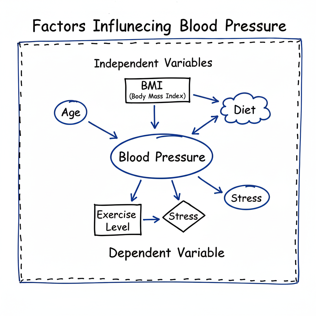
In biological and health sciences, data rarely follows a simple pattern. Organisms, populations, and diseases are influenced by numerous interrelated factors. For instance, blood pressure may depend on age, body weight, and cholesterol levels simultaneously. To model such multifactorial relationships, Multiple Regression Analysis becomes an essential statistical tool.
Multiple regression extends the concept of simple linear regression by incorporating two or more independent variables to predict a single dependent variable. It helps researchers quantify how much each predictor contributes to changes in the outcome variable while controlling for the effects of others. This makes it invaluable in epidemiology, clinical trials, genetics, and environmental biology.
What is Multiple Regression?
Multiple regression is a statistical technique used to explain or predict the value of a dependent (response) variable using several independent (predictor) variables.
It is represented by the following general equation:
Y=b0+b1X1+b2X2+…+bnXn+ε
Where:
- Y = Dependent variable
- X1,X2,…Xn = Independent variables
- b0 = Intercept (constant)
- b1,b2,…bn = Regression coefficients
- ε = Random error term
Each regression coefficient (bi) represents the change in the dependent variable for a one-unit change in Xi, keeping other variables constant.
Applications in Biostatistics
Multiple regression is widely used in biostatistics for both descriptive and predictive modeling. Common applications include:
| Field | Example of Use |
|---|---|
| Epidemiology | Predicting disease risk from lifestyle factors such as smoking, diet, and physical activity. |
| Clinical Research | Estimating patient outcomes (e.g., blood pressure or glucose level) from multiple physiological parameters. |
| Genetics | Studying the influence of multiple genes on a phenotype. |
| Environmental Health | Modeling the effect of pollutants, temperature, and humidity on respiratory illness. |
| Public Health | Predicting healthcare costs or resource use based on demographic and behavioral variables. |
Types of Multiple Regression
Multiple regression can be classified based on the nature of relationships and model complexity.
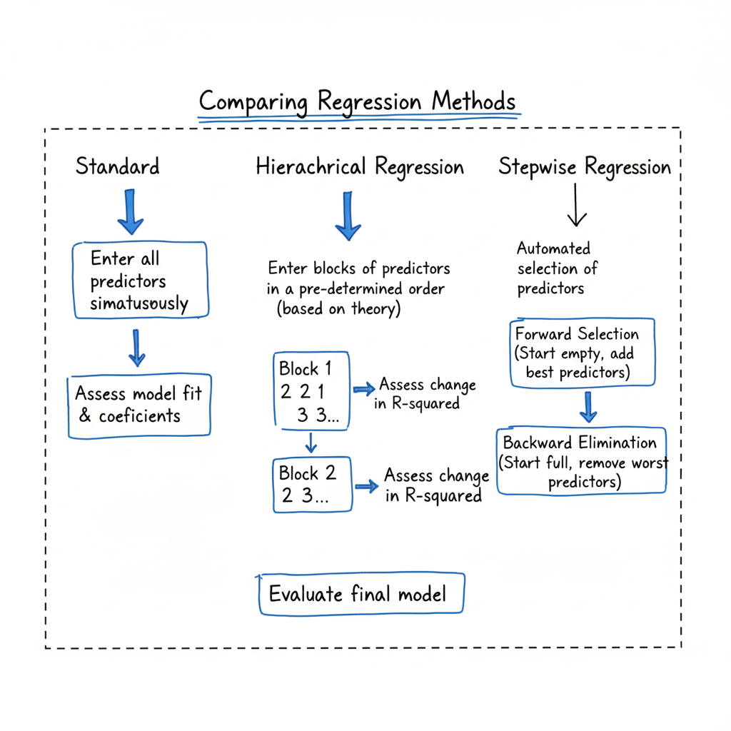
1. Standard (Simultaneous) Multiple Regression
All predictor variables are entered into the model simultaneously. The contribution of each variable is assessed while holding others constant.
2. Hierarchical (Sequential) Regression
Predictors are added in steps (blocks) based on theoretical or logical reasoning. It allows researchers to evaluate the incremental variance explained by new variables.
3. Stepwise Regression
An automated approach that adds or removes variables based on their statistical significance (p-value or contribution to R²). It helps in model optimization but may lead to overfitting if not used carefully.
Assumptions of Multiple Regression
To ensure valid results, multiple regression must satisfy the following assumptions:
| Assumption | Description | How to Check |
|---|---|---|
| Linearity | The relationship between dependent and each independent variable is linear. | Scatterplots and residual plots. |
| Independence of Errors | Observations are independent. | Durbin–Watson test. |
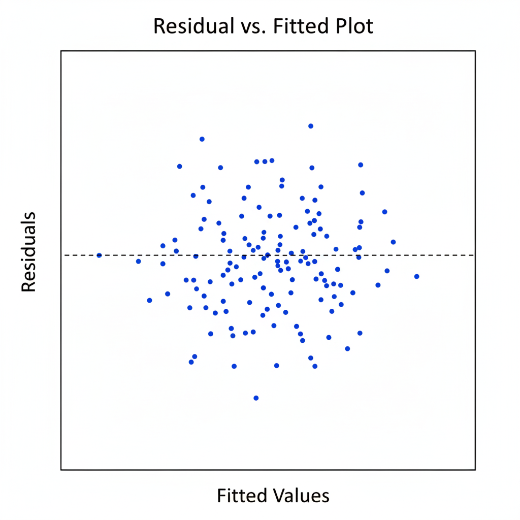
| Homoscedasticity | Equal variance of errors across predicted values. | Residual vs. fitted value plot. |
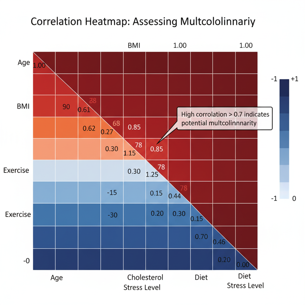
| Multicollinearity | Predictors are not highly correlated. | Variance Inflation Factor (VIF). |
| Normality of Errors | Residuals are normally distributed. | Histogram or Q-Q plot of residuals. |
Failure to meet these assumptions can lead to biased or inefficient estimates. Hence, diagnostic checking is a crucial part of regression analysis.
Interpretation of Regression Output
Once a multiple regression model is fitted, the output usually includes:
- Regression Coefficients (b₁, b₂, … bₙ): Indicate the direction and magnitude of relationships.
- R-squared (R²): Represents the proportion of variance in the dependent variable explained by all predictors.
- Adjusted R²: Adjusted for the number of predictors; more reliable for model comparison.
- p-values: Show whether the relationship between each predictor and outcome is statistically significant.
- Standard Error (SE): Reflects the accuracy of coefficient estimates.
Example Interpretation
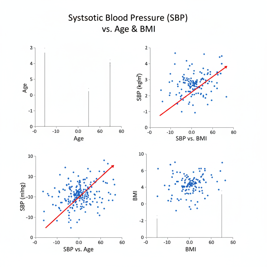
Consider the model predicting Systolic Blood Pressure (SBP) using Age (X₁) and BMI (X₂). SBP=80+0.5(Age)+1.2(BMI)
| Variable | Coefficient (b) | Std. Error | t-value | p-value |
|---|---|---|---|---|
| Intercept | 80.00 | 4.2 | 19.0 | 0.000 |
| Age | 0.50 | 0.10 | 5.0 | 0.001 |
| BMI | 1.20 | 0.25 | 4.8 | 0.002 |
Interpretation:
- For every one-year increase in age, SBP increases by 0.5 mmHg, holding BMI constant.
- For every one-unit increase in BMI, SBP increases by 1.2 mmHg, controlling for age.
- Both predictors significantly influence SBP (p < 0.05).
Evaluating Model Fit
1. Coefficient of Determination (R²)
R² measures how well the model explains variation in the dependent variable. For example, an R² of 0.72 means 72% of the variance in the outcome is explained by the predictors.
2. Adjusted R²
Used when comparing models with different numbers of predictors. It adjusts R² by penalizing unnecessary variables.
3. F-test
Tests the overall significance of the model—whether all regression coefficients are zero simultaneously.
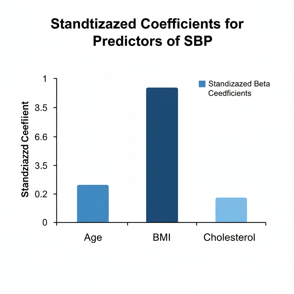
4. Standardized Coefficients (Beta values)
Enable comparison of the relative importance of each predictor.
Dealing with Multicollinearity
Multicollinearity occurs when predictors are highly correlated with one another. It can inflate standard errors and make coefficient estimates unstable.
Common Remedies
- Remove or combine correlated predictors.
- Use Principal Component Regression (PCR) or Partial Least Squares (PLS).
- Center the predictors by subtracting their means.
Model Validation
After fitting the regression model, validation ensures reliability and generalizability.
| Validation Method | Purpose |
|---|---|
| Cross-validation | Assess model performance on unseen data. |
| Residual analysis | Detect nonlinearity, heteroscedasticity, or outliers. |
| Cook’s Distance | Identify influential observations. |
| Q-Q plot | Check normality of residuals. |
Advantages of Multiple Regression
- Handles multiple predictors simultaneously.
- Controls for confounding variables.
- Provides predictive equations.
- Quantifies the strength and direction of relationships.
- Flexible for both continuous and categorical predictors (using dummy variables).
Limitations
- Sensitive to outliers and assumption violations.
- Interpretation becomes complex with many predictors.
- Multicollinearity can distort results.
- Requires a large sample size for stable estimates.
Example in Biological Research
A biostatistician investigates the effect of Age, BMI, and Cholesterol Level on Blood Pressure in 100 adults. After performing multiple regression:
Blood Pressure=70+0.45(Age)+1.1(BMI)+0.30(Cholesterol)
R² = 0.68, p < 0.001
Interpretation:
- The model explains 68% of variation in blood pressure.
- All predictors significantly contribute to changes in blood pressure.
- BMI has the highest effect size, indicating obesity as a key determinant.
Conclusion
Multiple regression analysis is a cornerstone of modern biostatistics, enabling researchers to explore complex relationships among biological, behavioral, and environmental variables. By incorporating multiple predictors, it provides a deeper understanding of the factors influencing health outcomes and biological processes.
However, careful attention must be paid to assumptions, model selection, and validation to ensure reliable results. With advancements in computational tools, multiple regression remains a powerful method for data-driven discovery in biological and health sciences.