Introduction
In biomedical and clinical laboratory research, a new analytical method must often be compared with an established reference method before it can be considered suitable for routine use. For example, a laboratory may introduce a new analyzer and need to determine whether its measurements are sufficiently comparable with those obtained from an existing reference analyzer.
One commonly used statistical technique for this purpose is Deming regression.
Unlike ordinary least-squares regression, Deming regression considers measurement error in both analytical methods. This makes it particularly useful for laboratory method-comparison studies where neither measurement procedure can reasonably be assumed to be completely error-free.
In this tutorial, we use MedCalc to demonstrate Deming regression using a biomedical analyzer dataset containing measurements from a reference analyzer and a new analyzer, together with duplicate measurements. The attached dataset contains measurements expressed in mg/dL.
The dataset contains 20 samples. Duplicate measurements are available for the reference analyzer for all 20 samples, while the duplicate measurement for the new analyzer is missing for Sample 16. Consequently, 19 complete duplicate pairs are available for assessing within-method analytical variation.
The purpose of this analysis is to demonstrate how Deming regression can be used to evaluate the relationship between a reference laboratory method and a new analytical method.
What Is Deming Regression?
Deming regression is a method-comparison regression technique that accounts for measurement error in both variables.
This is important in laboratory science because both the reference method and the new method can have analytical imprecision.
Suppose:
- X = Reference Analyzer
- Y = New Analyzer
Deming regression estimates the relationship between X and Y while considering measurement variation in both methods.
The resulting regression equation has the general form:
Y = Intercept + Slope × X
The two most important parameters are:
Intercept
The intercept provides information about a possible constant or additive difference between the methods.
Slope
The slope provides information about a possible proportional difference between the methods.
A slope close to 1 and an intercept close to 0 generally indicate a relationship close to the line of equality.
However, statistical results should always be evaluated together with clinical or analytical acceptance criteria.
Biomedical Dataset Used in This Example
The Excel file supplied for this tutorial contains the following variables:
| Variable | Description |
|---|---|
| Sample ID | Identification number |
| Reference Analyzer (mg/dL) | Primary reference measurement |
| Duplicate Reference Analyzer (mg/dL) | Duplicate reference measurement |
| New Analyzer (mg/dL) | Primary new-analyzer measurement |
| Duplicate New Analyzer (mg/dL) | Duplicate new-analyzer measurement |
Your dataset contains 20 samples.
Dataset
| Sample | Reference | Duplicate Reference | New Analyzer | Duplicate New |
|---|---|---|---|---|
| 1 | 82 | 83 | 84 | 85 |
| 2 | 91 | 92 | 94 | 95 |
| 3 | 98 | 96 | 100 | 99 |
| 4 | 105 | 104 | 108 | 105 |
| 5 | 112 | 113 | 115 | 114 |
| 6 | 120 | 121 | 122 | 123 |
| 7 | 128 | 129 | 131 | 130 |
| 8 | 135 | 134 | 137 | 138 |
| 9 | 143 | 144 | 146 | 147 |
| 10 | 150 | 151 | 153 | 154 |
| 11 | 158 | 159 | 161 | 160 |
| 12 | 166 | 167 | 168 | 169 |
| 13 | 175 | 178 | 178 | 179 |
| 14 | 184 | 182 | 186 | 187 |
| 15 | 193 | 194 | 196 | 195 |
| 16 | 202 | 201 | 204 | — |
| 17 | 215 | 214 | 218 | 219 |
| 18 | 228 | 225 | 231 | 232 |
| 19 | 240 | 239 | 243 | 244 |
| 20 | 255 | 256 | 258 | 259 |
Note: The missing value in Sample 16 is retained as missing rather than being replaced or estimated.
📥 Download the Example Data File
Why Are Duplicate Measurements Included?
Duplicate measurements are useful because they provide information about the analytical variation of each method.
For example, the difference between:
Reference Analyzer − Duplicate Reference Analyzer
provides information about repeatability of the reference method.
Similarly:
New Analyzer − Duplicate New Analyzer
provides information about repeatability of the new method.
In your dataset, the duplicate measurements are particularly useful because Deming regression can take measurement variability into account.
Coefficient of Variation in Your Dataset
Using the duplicate measurements, the within-method variation can be assessed.
For the reference analyzer, the duplicate differences give an estimated coefficient of variation of approximately 0.66%.
For the new analyzer, the corresponding coefficient of variation is approximately 0.53%, based on the 19 complete duplicate pairs.
| Method | Complete duplicate pairs | Approx. CV |
|---|---|---|
| Reference Analyzer | 20 | 0.66% |
| New Analyzer | 19 | 0.53% |
The relatively small CV values indicate low within-method analytical variation in this teaching dataset.
Importantly, a low CV demonstrates good repeatability but does not by itself establish agreement between the two methods.
How to Perform Deming Regression in MedCalc
Open your Excel dataset in MedCalc.
Then select:
Statistics → Method comparison & evaluation → Deming regression
The Deming regression dialog contains fields for the two methods and their duplicate measurements.
Method X
For Method X, select:
Reference Analyzer (mg/dL)
This represents the established or reference measurement procedure.
Duplicate
Select:
Duplicate Reference Analyzer (mg/dL)
This allows MedCalc to obtain information about the analytical variation of the reference method.
Method Y
For Method Y, select:
New Analyzer (mg/dL)
This represents the new analytical procedure being evaluated.
Duplicate
Select:
Duplicate New Analyzer (mg/dL)
The missing duplicate measurement for Sample 16 remains blank.
What Does the CV Option Mean?
The CV field allows the user to provide the coefficient of variation when duplicate measurements are not directly available.
If duplicate measurements are supplied, MedCalc can use them to estimate measurement variability.
This is especially useful for laboratory studies because analytical imprecision may differ between the reference and new methods.
Duplicate Measurements and CV
Duplicate measurements are useful when the investigator wants to estimate analytical variation within the methods.
The supplied MedCalc output reports:
| Method | Mean | Coefficient of Variation |
|---|---|---|
| X | 156.8158 | 0.66% |
| Y | 159.5526 | 0.53% |
These values are directly reported by MedCalc.
The coefficient of variation is relatively small for both methods in this example. The Y method has a CV of 0.53%, compared with 0.66% for X.
The CV describes relative variability, but it should not by itself be interpreted as evidence that one method is clinically interchangeable with the other.
Important Deming Regression Options
Scatter Diagram and Regression Line
This option displays the paired observations together with the fitted Deming regression line.
The graph allows the researcher to visually assess whether the observations follow a reasonably linear relationship.
Residuals
The residual plot shows the difference between observed and fitted values.
Residuals distributed approximately around zero without a strong systematic pattern are generally desirable.
A clear curved pattern, increasing spread, or clustering may suggest problems such as non-linearity or non-constant variability.
Duplicate Measurements
The duplicate fields allow MedCalc to incorporate replicate measurements when estimating the measurement-error characteristics of the two methods.
This is especially valuable in laboratory validation because analytical imprecision is rarely identical between instruments.
CV
The coefficient of variation can be supplied when duplicate measurements are not directly entered and the analytical variability is known.
CV is expressed as a percentage.
Results from the MedCalc Analysis
The supplied analysis contains 19 observations and reports a variance ratio of 1.5185.
The main Deming regression equation is:
y = 1.1220 + 1.0103x
The estimated intercept is 1.1220, while the slope is 1.0103.
Regression Results
| Parameter | Coefficient | Standard Error | 95% CI |
|---|---|---|---|
| Intercept | 1.1220 | 0.5555 | −0.04498 to 2.2890 |
| Slope | 1.0103 | 0.004010 | 1.0019 to 1.0187 |
Interpretation of the Intercept
The estimated intercept is 1.1220 mg/dL.
Its 95% confidence interval ranges from −0.04498 to 2.2890 mg/dL.
Because the confidence interval includes zero, the analysis does not provide strong statistical evidence of a non-zero constant bias.
Scientifically, this suggests that there is no clear evidence of a fixed additive difference between the two methods based on the intercept confidence interval.
Interpretation of the Slope
The estimated slope is 1.0103, with a 95% confidence interval of 1.0019 to 1.0187.
A slope of 1 would indicate that the two methods increase at the same rate.
The estimated slope is very close to 1, indicating a strong proportional relationship. However, the reported confidence interval lies slightly above 1.
Therefore, the result suggests a small proportional difference between the methods rather than a large systematic difference.
For example, using the fitted equation:
- At X = 100, predicted Y ≈ 102.15
- At X = 200, predicted Y ≈ 203.18
This illustrates the practical magnitude of the estimated difference.
Whether such a difference is clinically acceptable depends on the analyte, clinical decision limits, analytical performance specifications, and intended use of the measurement.
Pearson Correlation
MedCalc reports a Pearson correlation coefficient of:
r = 0.9999
with a 95% confidence interval from 0.9998 to 1.0000.
This indicates an extremely strong linear association between the two measurement methods.
However, an important scientific point should be emphasized:
A very high correlation does not automatically mean that two methods agree.
Two methods can correlate almost perfectly while maintaining a systematic bias. Therefore, the regression results should be interpreted alongside agreement analyses such as Bland–Altman analysis.
Interpretation of the Deming Regression Plot

The supplied regression graph shows the observations positioned close to the fitted regression line.
The plotted relationship is strongly linear, consistent with the extremely high Pearson correlation coefficient reported by MedCalc.
The regression equation displayed on the graph is approximately:
y = 1.122 + 1.010x
with n = 19.
The regression line is very close to the line of equality, indicating that the new analyzer produces measurements broadly similar to those obtained with the reference analyzer across the observed concentration range.
The small upward difference in the slope indicates that the new method tends to increase slightly faster than the reference method.
Residual Plot Interpretation
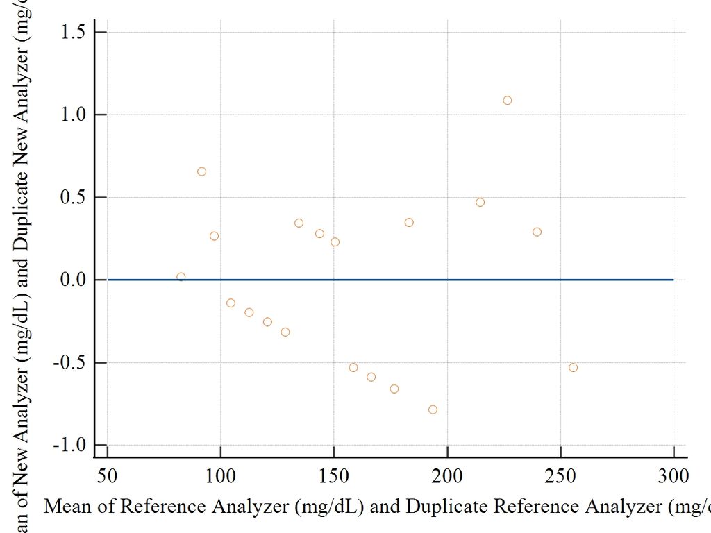
The residual graph provides another important diagnostic.
Residuals represent the deviations of individual observations from the fitted relationship.
In the supplied residual plot, observations are distributed on both sides of the zero reference line. There is no obvious large systematic departure from the fitted relationship.
This supports the visual impression that the Deming regression provides a good description of the paired measurements.
Nevertheless, researchers should inspect residuals carefully for:
- Curvature
- Increasing or decreasing spread
- Extreme observations
- Clustering
- Systematic positive or negative deviations
A residual pattern can reveal problems that may not be obvious from the correlation coefficient alone.
How to Report Deming Regression in a Scientific Journal
A concise journal-style result could be written as follows:
“Deming regression analysis was performed to evaluate the relationship between the new analyzer and the reference analyzer. A total of 19 paired observations were included. The regression equation was y = 1.1220 + 1.0103x, with an intercept of 1.1220 (95% CI, −0.04498 to 2.2890) and a slope of 1.0103 (95% CI, 1.0019–1.0187). The Pearson correlation coefficient was 0.9999 (95% CI, 0.9998–1.0000), indicating an extremely strong linear association between the methods. The intercept confidence interval included zero, whereas the slope was slightly greater than unity, suggesting minimal constant bias but a small proportional difference between the measurement methods.”
For a complete method-validation study, this interpretation should be supplemented by an assessment of clinical or analytical acceptability rather than relying on correlation alone.
Deming Regression Result Table for a Research Report
A convenient presentation format is:
| Statistical parameter | Result |
|---|---|
| Sample size | 19 |
| Mean of reference method | 156.8158 |
| CV of reference method | 0.66% |
| Mean of new method | 159.5526 |
| CV of new method | 0.53% |
| Variance ratio | 1.5185 |
| Intercept | 1.1220 |
| 95% CI for intercept | −0.04498 to 2.2890 |
| Slope | 1.0103 |
| 95% CI for slope | 1.0019 to 1.0187 |
| Pearson correlation | 0.9999 |
| 95% CI for correlation | 0.9998 to 1.0000 |
Advantages of Deming Regression
Deming regression is particularly useful because it:
- Accounts for measurement error in both methods.
- Is appropriate for analytical method comparison.
- Can incorporate information about replicate measurements.
- Provides estimates of intercept and slope.
- Provides confidence intervals.
- Helps identify potential constant and proportional differences.
- Produces a useful graphical representation of the relationship.
Important Limitation
Deming regression should not be interpreted as proof of clinical interchangeability.
A high correlation and a regression line close to the equality line are encouraging, but method agreement should also be evaluated using appropriate agreement techniques.
For example, Bland–Altman analysis can help determine the magnitude and limits of differences between two measurement methods.
Therefore, a strong biomedical method-comparison study may combine:
Deming regression + Bland–Altman analysis + analytical performance criteria + clinical acceptability.
Conclusion
Deming regression in MedCalc is a valuable technique for comparing two quantitative biomedical measurement methods when measurement error exists in both methods.
In the supplied example, 19 observations were analyzed. The fitted regression equation was y = 1.1220 + 1.0103x, with an intercept confidence interval that included zero and a slope very close to one. The Pearson correlation coefficient of 0.9999 demonstrated an extremely strong linear association.
The results indicate a very strong relationship between the reference and new analyzer measurements, with only a small estimated proportional difference. However, correlation alone cannot establish agreement or clinical interchangeability.
For biomedical and laboratory research, Deming regression is therefore best viewed as an important component of a broader method-comparison and analytical validation strategy.