Introduction
In many biological, agricultural, medical, and experimental studies, researchers compare several groups to determine whether a treatment produces a difference in the outcome. A simple One Way ANOVA can be used for this purpose. However, sometimes the outcome is also influenced by an additional continuous variable.
For example, plant growth after treatment may be strongly related to the initial plant growth before treatment. If the initial growth values are different among observations, a direct comparison of final growth may not provide a complete picture of the treatment effect.
This is where Analysis of Covariance (ANCOVA) becomes useful. ANCOVA combines the principles of ANOVA and regression analysis. It compares group means after statistically adjusting for the influence of a continuous covariate.
What is One Way ANCOVA?
One Way ANCOVA is a statistical technique used to examine whether the means of two or more independent groups differ significantly after controlling for the effect of a continuous covariate.
The term “One Way” means that there is one categorical independent variable or factor. In this analysis, the factor is the fertilizer treatment.
ANCOVA can be expressed conceptually as:
Dependent Variable = Group Effect + Covariate Effect + Error
The main purpose is to determine whether the group factor still explains a significant amount of variation in the dependent variable after the covariate has been taken into account.
Concept of ANCOVA
The main concept behind ANCOVA is statistical adjustment.
Suppose one plant starts with a much higher growth value than another plant. It may naturally have a higher final growth value even without a treatment effect. By including the initial growth measurement as a covariate, ANCOVA adjusts the final growth comparison for the influence of the baseline measurement.
This gives a more meaningful comparison among treatment groups.
The three important components are:
Factor: The categorical variable defining the groups.
Covariate: A continuous variable that may influence the dependent variable.
Dependent variable: The continuous outcome being compared among groups.
One Way ANCOVA in SPSS: Procedure
The analysis can be performed in SPSS using the following procedure:
Analyze → General Linear Model → Univariate
Then enter:
Dependent Variable: After_Plants_Growth
Fixed Factor: Factor
Covariate: Befor_Plants_Growth
Under Options, descriptive statistics, homogeneity tests, and effect sizes can be selected.
The supplied SPSS syntax uses Type III sums of squares, includes the factor and covariate, and also includes the Factor × Befor_Plants_Growth interaction. The significance level is set at 0.05.
Descriptive Statistics
Before interpreting the ANCOVA, it is useful to examine the descriptive statistics.
The four fertilizer groups show different raw mean values for After_Plants_Growth. The CF+OM group has the highest mean, while the Control group has the lowest mean.
Table 1. Descriptive Statistics for After_Plants_Growth
| Factor | Mean | Std. Deviation | N |
|---|---|---|---|
| Control | 78.60 | 9.03 | 10 |
| CF | 83.00 | 12.61 | 10 |
| OM | 89.30 | 14.33 | 10 |
| CF+OM | 102.50 | 9.48 | 10 |
| Total | 88.35 | 14.38 | 40 |
The descriptive results indicate that the observed average after-growth increases from Control to CF, OM, and finally CF+OM.
However, these are unadjusted means. A higher raw mean does not automatically mean that the treatment effect is statistically significant after adjusting for the covariate.
Assumptions of One Way ANCOVA
Several assumptions should be considered before interpreting an ANCOVA.
1. Independence of observations
Each observation should be independent of the others. This assumption mainly depends on how the experiment was designed. It cannot be fully established from the SPSS output alone.
2. Continuous dependent variable and covariate
The dependent variable and covariate should be measured on an appropriate continuous scale. In this analysis, After_Plants_Growth is the outcome and Befor_Plants_Growth is the continuous covariate.
3. Homogeneity of regression slopes
One important ANCOVA assumption is that the relationship between the covariate and dependent variable should be similar across groups.
This is examined using the Factor × Befor_Plants_Growth interaction.
The interaction was:
F(3, 32) = 0.197, p = .898, partial η² = .018
Since p = .898 > .05, the interaction is not statistically significant. Therefore, there is no significant evidence that the relationship between before-growth and after-growth differs among the fertilizer groups.
4. Homogeneity of error variances
Levene’s test is used to examine whether the error variances are approximately equal across groups.
The result was:
F(3, 36) = 5.744, p = .003
Because p < .05, the assumption of equal error variances is not supported.
Therefore, the standard ANCOVA result should be interpreted with some caution. This assumption violation should be mentioned clearly in a research report or thesis.
Table 2. Assumption Tests
| Test | F | df1 | df2 | Sig. | Interpretation |
|---|---|---|---|---|---|
| Levene’s Test | 5.744 | 3 | 36 | .003 | Significant; equal variances not supported |
| Factor × Befor_Plants_Growth | 0.197 | 3 | 32 | .898 | Non-significant; slope assumption supported |
Main One Way ANCOVA Result
The main ANCOVA result is presented in the Tests of Between-Subjects Effects table.
The corrected model was statistically significant:
F(7, 32) = 48.406, p < .001, partial η² = .914
The model produced:
R² = .914
Adjusted R² = .895
This indicates that approximately 91.4% of the variation in After_Plants_Growth is explained by the variables included in the model.
The most important finding concerns the covariate.
Effect of Befor_Plants_Growth
The covariate was highly significant:
F(1, 32) = 158.736, p < .001, partial η² = .832
This indicates that Befor_Plants_Growth is a very strong predictor of After_Plants_Growth.
The large partial eta squared value of .832 shows that the covariate accounts for a substantial amount of unique variability in the dependent variable.
Effect of Fertilizer Factor
After adjusting for Befor_Plants_Growth, the fertilizer factor was not statistically significant:
F(3, 32) = 0.370, p = .775, partial η² = .033
Because p = .775 > .05, the null hypothesis is not rejected.
Therefore, the supplied ANCOVA does not provide statistically significant evidence of a difference among the four fertilizer groups in adjusted After_Plants_Growth.
This is an important distinction from the descriptive results. Although CF+OM has the highest raw mean, that raw difference is not statistically significant after controlling for baseline plant growth.
Factor × Befor_Plants_Growth Interaction
The interaction was:
F(3, 32) = 0.197, p = .898, partial η² = .018
This non-significant interaction supports the assumption of homogeneous regression slopes.
Table 3. Tests of Between-Subjects Effects
| Source | Type III Sum of Squares | df | Mean Square | F | Sig. | Partial η² |
|---|---|---|---|---|---|---|
| Corrected Model | 7372.820 | 7 | 1053.260 | 48.406 | <.001 | .914 |
| Intercept | 106.545 | 1 | 106.545 | 4.897 | .034 | .133 |
| Factor | 24.122 | 3 | 8.041 | 0.370 | .775 | .033 |
| Befor_Plants_Growth | 3453.891 | 1 | 3453.891 | 158.736 | <.001 | .832 |
| Factor × Befor_Plants_Growth | 12.866 | 3 | 4.289 | 0.197 | .898 | .018 |
| Error | 696.280 | 32 | 21.759 | — | — | — |
R² = .914; Adjusted R² = .895.
Figure 1. Before and After Plant Growth by Fertilizer Group
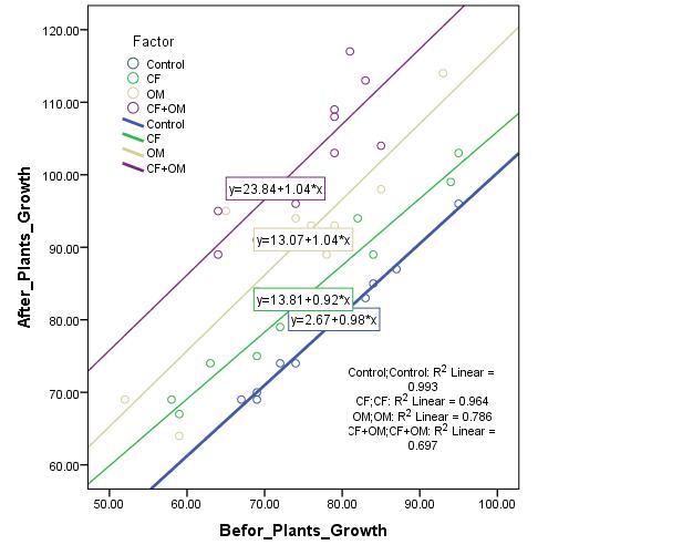
The graph indicates a clear positive relationship between before-treatment and after-treatment plant growth. As before-growth increases, after-growth generally also increases.
The fitted regression lines displayed in the figure are approximately:
Control: y = 2.67 + 0.98x, R² = .993
CF: y = 13.81 + 0.92x, R² = .964
OM: y = 13.07 + 1.04x, R² = .786
CF+OM: y = 23.84 + 1.04x, R² = .697
The figure therefore provides a visual explanation for the strong statistical effect of the covariate. The formal interaction test, however, is non-significant, so the numerical differences among the slopes should not be interpreted as statistically significant differences in regression slopes.
Interpretation of One Way ANCOVA Result
The results need to be interpreted carefully by separating the descriptive findings from the adjusted inferential findings.
The raw mean of the CF+OM group is 102.50, which is considerably higher than the Control mean of 78.60. At first glance, this may suggest that the combined fertilizer treatment produces greater plant growth.
However, ANCOVA controls for Befor_Plants_Growth, and this covariate has a very strong statistical effect:
F(1,32) = 158.736, p < .001, partial η² = .832.
After adjusting for this baseline variable, the fertilizer factor is no longer statistically significant:
F(3,32) = 0.370, p = .775, partial η² = .033.
Thus, the apparent differences in the raw group means cannot be interpreted as a statistically confirmed fertilizer effect based on this ANCOVA.
The covariate has a very large partial eta squared of .832, whereas the factor has only .033. In practical terms, the model indicates that baseline plant growth is much more influential than fertilizer group in explaining the variability in the final measurement. The overall model has a high R² because it captures this strong baseline-outcome relationship.
The assumption results should also be included in the interpretation. The Factor × Befor_Plants_Growth interaction is non-significant (p = .898), supporting the homogeneity-of-regression-slopes assumption. In contrast, Levene’s test is significant (p = .003), indicating unequal error variances among the groups.
Therefore, the ANCOVA result should be reported with appropriate caution rather than simply stating that the treatments are equivalent.
Dataset Download
Download One Way ANCOVA Dataset
Conclusion
The One Way ANCOVA in SPSS demonstrates that Befor_Plants_Growth has a strong and statistically significant relationship with After_Plants_Growth. The overall model is highly significant and explains 91.4% of the variation in the dependent variable.
Although the descriptive results show that the CF+OM group has the highest raw mean after-growth (102.50), the main fertilizer factor is not statistically significant after controlling for baseline plant growth:
F(3,32) = 0.370, p = .775, partial η² = .033.
Therefore, the appropriate conclusion is:
After controlling for Befor_Plants_Growth, there is no statistically significant difference in After_Plants_Growth among the Control, CF, OM, and CF+OM fertilizer groups.
The Factor × Befor_Plants_Growth interaction is non-significant, supporting the homogeneity-of-regression-slopes assumption. However, Levene’s test is significant, indicating a violation of the equal-variance assumption. Consequently, the standard ANCOVA finding should be interpreted cautiously and the variance assumption should be clearly acknowledged in a scientific report or thesis.