Passing-Bablok Regression in MedCalc is a useful statistical approach for evaluating whether two analytical measurement methods produce comparable results. It is particularly relevant in laboratory and biomedical research when a new analyzer or measurement procedure is compared with an established reference method.
In this tutorial, the Passing-Bablok Regression procedure in MedCalc is demonstrated using Reference Analyzer (mg/dL) as Variable X and New Analyzer (mg/dL) as Variable Y. The analysis contains 20 observations. The MedCalc report confirms these variable assignments and the sample size of 20.
What is Passing-Bablok Regression?
Passing-Bablok regression is a regression technique commonly used for method comparison studies. It evaluates the relationship between measurements obtained from two analytical methods without relying on the same assumptions as ordinary least-squares regression.
The method produces two particularly important parameters:
- Intercept (A) – used to evaluate constant differences or constant bias.
- Slope (B) – used to evaluate proportional differences or proportional bias.
The general regression equation is:
Y = A + B × X
where:
- Y = measurement obtained using the new or comparison method
- X = measurement obtained using the reference method
- A = intercept
- B = slope
For method comparison, an intercept close to 0 and a slope close to 1 generally indicate that the two methods are closely aligned. However, the confidence intervals are important because the estimated value alone does not determine whether a statistically meaningful difference exists.
Concept of Passing-Bablok Regression
The main objective of Passing-Bablok regression is to determine whether two measurement methods can be considered comparable across the measurement range.
Two types of systematic differences are especially important.
1. Constant difference
A constant difference occurs when one method consistently produces measurements that are higher or lower than the other method by approximately the same amount.
This is evaluated using the intercept.
- Intercept = 0 → no constant difference suggested.
- Confidence interval excludes 0 → evidence of a constant difference.
- Confidence interval includes 0 → no statistically demonstrated constant difference.
2. Proportional difference
A proportional difference occurs when the difference between methods changes according to the magnitude of the measurement.
This is evaluated using the slope.
- Slope = 1 → no proportional difference suggested.
- Confidence interval excludes 1 → evidence of proportional difference.
- Confidence interval includes 1 → no statistically demonstrated proportional difference.
Therefore, both the intercept and slope should be interpreted together.
Passing-Bablok Regression Options in MedCalc
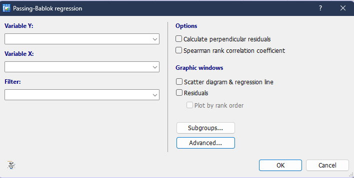
Variable Y
Variable Y represents the measurements obtained from the new or comparison method.
For this analysis:
Variable Y = New Analyzer (mg/dL)
The MedCalc report confirms this assignment.
Variable X
Variable X represents the reference or comparison method.
For this analysis:
Variable X = Reference Analyzer (mg/dL)
The report identifies Reference Analyzer as Variable X.
Filter
The Filter option can be used when only a specific subgroup or selected portion of the dataset should be analyzed.
For the present analysis, no specific filtering was applied.
Calculate perpendicular residuals
This option calculates residuals perpendicular to the regression line rather than using only vertical distances.
Perpendicular residuals can be useful for method-comparison visualization because both measurement axes are considered in relation to the fitted line.
Spearman rank correlation coefficient
This option provides the Spearman rank correlation coefficient, which evaluates the strength of the monotonic association between the two variables.
It should not be interpreted as a direct measure of agreement. Two methods can show a very strong correlation while still having clinically important systematic differences.
Scatter diagram & regression line
This option produces the main method-comparison scatter diagram.
The graph displays the observed measurements together with the Passing-Bablok regression line and the identity line.
The identity line represents perfect equality between the two methods.
Residuals
The Residuals option generates a residual plot that helps identify observations that deviate from the fitted regression relationship.
Residual plots can be particularly useful for identifying unusual observations or patterns that may not be obvious in the main scatter diagram.
Plot by rank order
The rank-order residual plot presents residuals according to the rank of the observations. This can help visualize unusual observations and systematic patterns.
Subgroups
The Subgroups option can be used when the dataset contains a categorical grouping variable. Different subgroups can then be displayed separately in the analysis or graphical output.
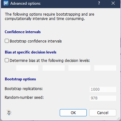
Advanced options
The Advanced options provide additional procedures, including:
- Bootstrap confidence intervals
- Bias estimation at specified decision levels
- Bootstrap replications
- Random-number seed
Bootstrap procedures can be useful when confidence intervals for regression parameters are required through resampling.
Results of Passing-Bablok Regression
The uploaded MedCalc output contains 20 observations. The Reference Analyzer values range from 82.0000 to 255.0000 mg/dL, while the New Analyzer values range from 1.0000 to 258.0000 mg/dL.
Table 1. Descriptive statistics from the Passing-Bablok analysis
| Statistic | Reference Analyzer (X) | New Analyzer (Y) |
|---|---|---|
| Sample size | 20 | 20 |
| Lowest value | 82.0000 | 1.0000 |
| Highest value | 255.0000 | 258.0000 |
| Arithmetic mean | 159.0000 | 157.5000 |
| Median | 154.0000 | 157.0000 |
| Standard deviation | 51.5057 | 60.7389 |
| Standard error of mean | 11.5170 | 13.5816 |
Passing-Bablok Regression Equation
The MedCalc output gives the following regression equation:
Y = 3.000000 + 1.000000 X
Thus, for this dataset:
New Analyzer = 3.000000 + 1.000000 × Reference Analyzer
The regression results are summarized below.
Table 2. Passing-Bablok regression results
| Parameter | Estimate | 95% CI | Interpretation |
|---|---|---|---|
| Intercept (A) | 3.0000 | 1.5892 to 3.0000 | Constant difference indicated |
| Slope (B) | 1.0000 | 1.0000 to 1.0064 | No statistically demonstrated proportional difference |
| Residual SD | 14.0060 | — | Residual variability |
| ±1.96 RSD interval | — | −27.4517 to 27.4517 | Approximate residual interval |
Interpretation of the Intercept
The estimated intercept is:
A = 3.0000
with a 95% confidence interval of:
1.5892 to 3.0000
Because this confidence interval does not include 0, the results indicate a statistically demonstrated constant difference between the methods in this dataset.
In practical terms, the New Analyzer is estimated to have a positive constant offset relative to the Reference Analyzer.
The intercept should therefore be reported rather than interpreting the two methods as having complete equality.
Interpretation of the Slope
The estimated slope is:
B = 1.0000
with a 95% confidence interval of:
1.0000 to 1.0064
The confidence interval includes 1.0000. Therefore, there is no statistically demonstrated proportional difference between the two methods based on this Passing-Bablok analysis.
This means the relationship between the methods does not provide evidence that the difference systematically increases or decreases with measurement magnitude.
Scatter Plot Interpretation
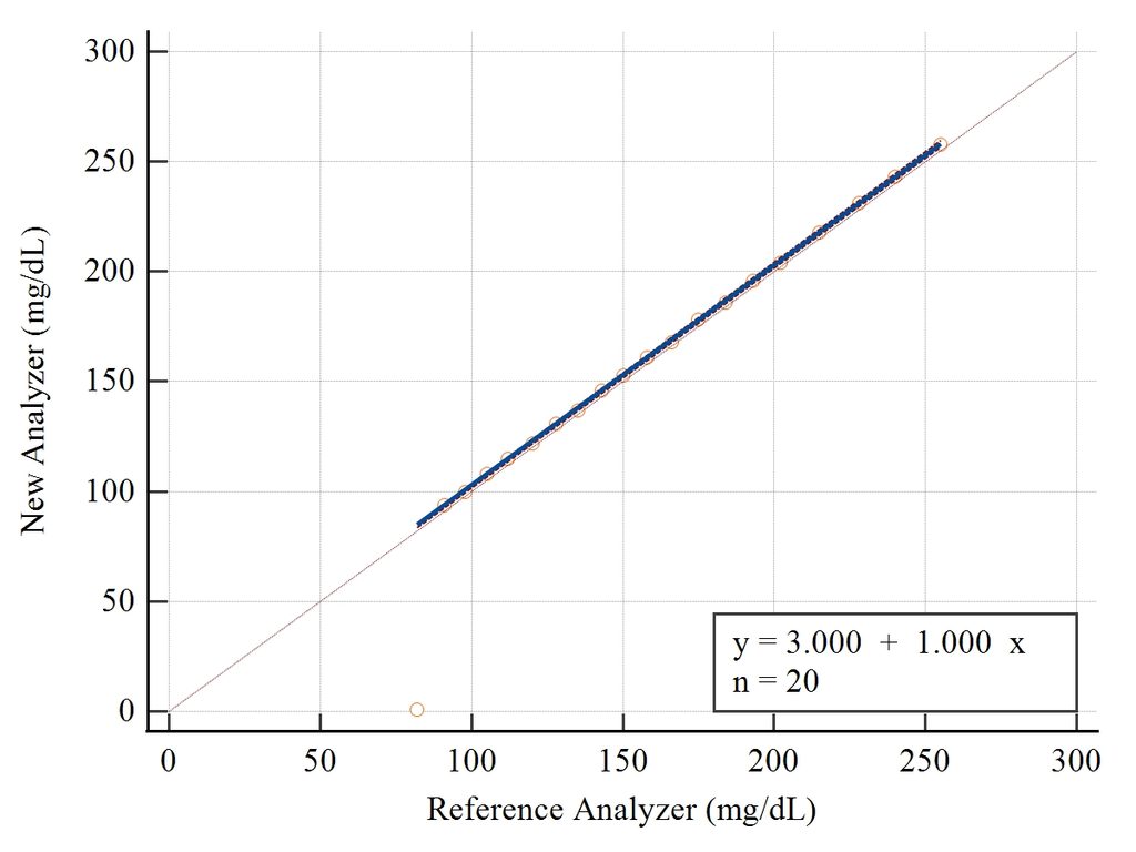
The observations are concentrated very closely around the regression line across most of the measurement range. The identity line is also shown, allowing visual comparison between the two analytical methods.
The regression equation displayed on the graph is:
y = 3.000 + 1.000x
with n = 20.
Most observations closely follow the expected linear relationship. However, one observation appears far below the main group, near a New Analyzer value of approximately 1 mg/dL. This unusual observation should not automatically be deleted. It should first be checked against the original data and, if applicable, the laboratory record.
The scatter plot therefore demonstrates a strong overall linear relationship while also highlighting an unusual observation that deserves attention.
Residual Plot Interpretation
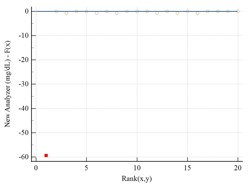
Most observations are clustered close to the zero residual line. However, one observation produces a very large negative residual, approximately −60 mg/dL, which corresponds to the isolated observation visible in the scatter plot.
The residual standard deviation reported by MedCalc is 14.0060, and the ±1.96 RSD interval is −27.4517 to 27.4517.
This residual plot is useful because it makes the unusual observation much easier to recognize than from the regression equation alone.
Spearman Rank Correlation
The MedCalc output reports:
Spearman correlation coefficient = 1.000
P < 0.0001
This indicates an extremely strong monotonic association between the rankings of the two measurement methods, and the association is statistically significant.
However, an important point should be emphasized:
A high correlation does not automatically mean that two measurement methods agree.
Correlation evaluates association, whereas method-comparison analysis should also examine systematic differences, regression parameters, residual behavior, and clinically or analytically acceptable differences.
Linear Model Validity
The MedCalc output includes a section for the Cusum test for linearity, but no numerical result is displayed in the supplied report.
Therefore, a specific conclusion about the Cusum linearity test should not be made from this report alone.
The graphical results nevertheless show that the majority of observations follow a close linear pattern, while the isolated low New Analyzer observation produces a prominent residual.
Overall Interpretation
The Passing-Bablok regression produced:
- Intercept = 3.0000
- 95% CI = 1.5892–3.0000
- Slope = 1.0000
- 95% CI = 1.0000–1.0064
- Spearman correlation = 1.000
- P < 0.0001
- Residual SD = 14.0060
- n = 20
The intercept confidence interval excludes zero, indicating evidence of a constant difference. In contrast, the slope confidence interval includes one, indicating no statistically demonstrated proportional difference.
The scatter plot demonstrates a strong linear relationship between the Reference Analyzer and New Analyzer measurements. The residual plot identifies one markedly unusual observation that should be investigated before drawing a final conclusion about analytical performance.
⬇️ Download Passing-Bablok Regression Dataset – Excel
Conclusion
Passing-Bablok regression provides a valuable approach for comparing two analytical measurement methods. In the present MedCalc example, the analysis included 20 observations and produced a regression equation of Y = 3.0000 + 1.0000X. The intercept confidence interval indicated a constant difference, whereas the slope confidence interval did not demonstrate a proportional difference.
The Spearman correlation was 1.000 with P < 0.0001, demonstrating an extremely strong monotonic relationship. However, correlation should not be used alone to establish agreement.
The scatter plot and residual plot provide additional information, particularly the prominent unusual observation. Consequently, Passing-Bablok regression should be interpreted together with graphical assessment and other appropriate method-comparison procedures when evaluating whether a new analytical method is suitable for practical use.