Introduction

Cluster analysis is one of the most popular unsupervised machine learning techniques used in biology, ecology, microbiology, genetics, medicine, and many other scientific disciplines. Unlike supervised learning methods, clustering does not require predefined class labels. Instead, it identifies natural groupings among samples based on their similarity.

A Cluster Dendrogram is the graphical representation of hierarchical clustering. It visually illustrates how observations are merged into clusters step by step. Researchers use dendrograms to identify similar biological samples, classify organisms, analyze gene expression data, compare microbial communities, and understand relationships among observations.

In this tutorial, you will learn how to create a professional Cluster Dendrogram in RStudio using an Excel dataset. Every step is explained in detail—from importing the data to interpreting the final dendrogram.

What is Hierarchical Clustering?

Hierarchical clustering is an unsupervised statistical method that groups observations according to their similarity or distance.

Instead of assigning observations directly into a fixed number of clusters, hierarchical clustering builds a hierarchy of clusters.

The output is represented as a tree diagram called a dendrogram.

Types of Hierarchical Clustering

1. Agglomerative Clustering (Bottom-Up)

This is the most commonly used method.

Each sample starts as an individual cluster.

The algorithm repeatedly merges the two closest clusters until only one cluster remains.

Your R script uses this approach through the hclust() function.

2. Divisive Clustering (Top-Down)

The opposite approach.

All observations start in one large cluster.

The algorithm repeatedly divides the clusters into smaller groups.

What is a Dendrogram?

A dendrogram is a tree-like diagram showing the hierarchical relationships among observations.

Each branch represents one sample or one cluster.

The vertical axis (Height) indicates the dissimilarity or distance at which clusters merge.

Smaller heights indicate greater similarity.

Larger heights indicate greater differences.

Applications of Cluster Dendrogram

Cluster dendrograms are widely used in:

• Gene expression analysis
• Microbial diversity studies
• Ecology
• Biodiversity research
• Medical diagnosis
• Plant taxonomy
• Animal classification
• Environmental science
• Soil microbiology
• Agricultural research

Dataset Used

The dataset contains multiple biological samples stored in an Excel workbook. One column, named Sample, contains the sample identifiers, while the remaining columns contain numerical variables used for clustering. The script converts the Sample column into row names before analysis.

Step 1 – Clear the Workspace

Before starting the analysis, remove all existing objects from the R environment.

rm(list = ls())

Why?

This avoids conflicts with variables from previous analyses and ensures a clean workspace.

Step 2 – Load Required Package

library(readxl)

Why?

The readxl package allows RStudio to read Excel (.xlsx) files directly.

Step 3 – Import Excel Dataset

bio_data <- read_excel(file.choose())

Explanation

• Opens a file browser.
• Lets you select the Excel dataset.
• Imports the data into R as bio_data.

You can preview the imported data using:

head(bio_data)
View(bio_data)

These commands display the first few rows and the full dataset for verification.

Step 4 – Set Sample Names as Row Names

The script converts the imported object to a data frame, assigns the values in the Sample column as row names, and then removes the Sample column from the analysis data. This ensures that only numeric variables are used during clustering while the sample names appear as labels in the dendrogram.

Step 5 – Standardize the Data

bio_scaled <- scale(bio_df)

Why Standardization?

Biological variables often have different measurement units.

For example:

• pH
• Temperature
• Biomass
• Cell count

Without scaling, variables with larger numerical ranges dominate the distance calculation.

Standardization converts variables to a common scale (mean = 0, standard deviation = 1), making each variable contribute equally.

Step 6 – Calculate Euclidean Distance

dist_matrix <- dist(
bio_scaled,
method="euclidean")

What is Euclidean Distance?

Euclidean distance measures the straight-line distance between two samples.

Smaller distances indicate that two samples are very similar.

Larger distances indicate greater differences.

The script computes this distance matrix using the standardized data.

Step 7 – Perform Hierarchical Clustering

hc <- hclust(
dist_matrix,
method="complete")

Complete Linkage Method

Complete linkage calculates the distance between clusters using the farthest pair of observations.

Advantages include:

• Produces compact clusters
• Less sensitive to chaining
• Frequently used in biological research

The result is stored in the object hc.

Step 8 – Plot the Cluster Dendrogram

The script then plots the dendrogram using the hierarchical clustering object. It sets the main title to Cluster Dendrogram, labels the vertical axis as Height, removes the default x-axis label and subtitle, keeps all branches aligned with hang = -1, and uses readable text size with cex = 1.

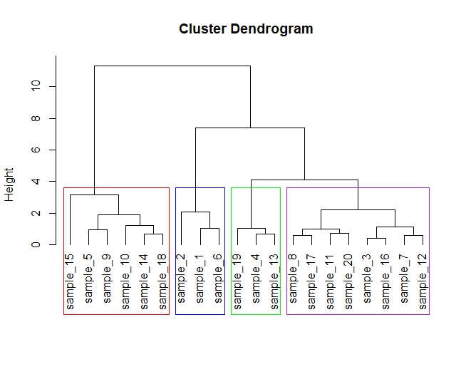
The resulting figure shows how samples are progressively merged into larger clusters based on similarity.

plot(
  hc,
  main = "Cluster Dendrogram",
  xlab = "",
  sub = "",
  ylab = "Height",
  hang = -1,
  cex = 1
)

Step 9 – Draw Cluster Boxes

The final step highlights the clusters by drawing colored rectangles around them.

The script specifies:

• Number of clusters = 4
• Border colors = Red, Blue, Green, and Purple

This makes the final dendrogram easier to interpret visually.

rect.hclust(
  hc,
  k = 4,
  border = c("red","blue","green","purple")
)

Understanding the Dendrogram

• Four colored rectangles indicate four major clusters.
• Samples inside the same colored box are more similar to each other than to samples in other boxes.
• Short branch lengths represent highly similar samples.
• Long branch lengths indicate greater differences between clusters.
• The y-axis (Height) represents the distance at which clusters merge.
• Clusters that merge at lower heights are more alike than those joining at higher heights.

This visualization helps researchers quickly identify groups of related biological samples.

Interpretation of the Cluster Dendrogram

The cluster dendrogram illustrates the hierarchical relationships among the 20 biological samples based on their measured characteristics. In this analysis, hierarchical agglomerative clustering was performed using Euclidean distance as the similarity measure and the complete linkage method to determine inter-cluster distances. The resulting dendrogram provides a visual representation of how individual samples are progressively merged into larger clusters according to their similarity.

The horizontal axis (X-axis) displays the sample identifiers (Sample_1 to Sample_20). Each label corresponds to one biological sample included in the analysis. Samples positioned next to each other in the dendrogram are not necessarily similar; rather, their similarity is determined by the branching pattern and the height at which they merge.

The vertical axis (Height) represents the dissimilarity (or linkage distance) between samples or clusters during the clustering process. Lower heights indicate greater similarity, whereas higher heights indicate greater dissimilarity. Therefore, samples that merge at a small height possess very similar characteristics, while clusters that merge at larger heights are considerably more distinct.

Cluster Formation

Based on the selected cut-off level (k = 4), the dendrogram is divided into four major clusters, each enclosed by a different colored rectangle.

Cluster 1 (Red)

This cluster contains:

• Sample_15
• Sample_5
• Sample_9
• Sample_10
• Sample_14
• Sample_18

These six samples merge at relatively low linkage heights, indicating that they exhibit a high degree of similarity across the measured biological variables. The short branch lengths within this cluster suggest relatively homogeneous characteristics and limited variation among its members.

Cluster 2 (Blue)

This cluster contains:

• Sample_2
• Sample_1
• Sample_6

This is a compact cluster composed of three samples. The branches connecting these samples occur at low heights, indicating that they are highly similar. Because this cluster contains fewer samples than the others, it may represent a distinct subgroup sharing a unique combination of biological characteristics.

Cluster 3 (Green)

This cluster contains:

• Sample_19
• Sample_4
• Sample_13

These three samples form another well-defined cluster. Their close linkage suggests that they share similar measurements and differ substantially from the samples in the remaining clusters.

Cluster 4 (Purple)

This cluster contains:

• Sample_8
• Sample_17
• Sample_11
• Sample_20
• Sample_3
• Sample_16
• Sample_7
• Sample_12

This is the largest cluster in the dataset. Although all eight samples belong to the same major group, several smaller subclusters can be observed within it. These subclusters indicate varying degrees of similarity among individual samples while still maintaining an overall relationship that distinguishes them from the other three clusters.

Interpretation of Branch Lengths

One of the most important aspects of dendrogram interpretation is the branch height.

Short Branches

Samples connected by short branches have very small Euclidean distances.

This indicates:

• High similarity
• Comparable biological characteristics
• Minimal variation between observations

For example, within each colored cluster, several samples merge at heights below approximately 2 units, indicating strong similarity.

Long Branches

Long branches indicate that larger distances exist between groups.

This suggests:

• Greater biological variation
• Lower similarity
• Distinct cluster composition

For example, the final branches joining the four major clusters occur at much higher linkage distances, indicating that these groups are substantially different from one another.

Hierarchical Merging Process

The dendrogram follows an agglomerative (bottom-up) clustering strategy.

Initially,

• every sample is treated as an independent cluster.

Next,

• the two most similar samples are merged.

Then,

• the algorithm repeatedly combines the closest clusters.

Finally,

• all samples become part of one large hierarchical tree.

This hierarchical merging process allows researchers to observe relationships at multiple levels of similarity rather than forcing observations into predefined groups.

Biological Interpretation

From a biological perspective, the four identified clusters suggest that the samples can be classified into four distinct groups based on their measured variables.

Samples within the same cluster are expected to possess comparable biological, ecological, physiological, or biochemical characteristics. Such similarities may arise from common environmental conditions, genetic relationships, experimental treatments, or shared phenotypic traits.

Conversely, samples belonging to different clusters exhibit greater dissimilarity, indicating substantial differences in their underlying characteristics.

The dendrogram therefore provides valuable insights into the natural grouping of biological samples and serves as an effective exploratory tool for identifying patterns within complex datasets.

Interpretation of the Height Scale

The height values shown on the Y-axis represent the linkage distance at which clusters are combined.

• Height ≈ 0–2: Very high similarity among samples.
• Height ≈ 2–5: Moderate similarity; small clusters begin to merge.
• Height > 5: Larger clusters merge, indicating increased dissimilarity.
• Maximum height (around 11 in this example): Final merging of all clusters into a single hierarchical structure, representing the greatest dissimilarity observed in the dataset.

Thus, the greater the merging height, the less similar the clusters are.

Overall Scientific Interpretation

The hierarchical clustering analysis successfully classified the twenty biological samples into four major clusters using Euclidean distance and the complete linkage algorithm. Samples grouped within the same cluster exhibit high similarity, whereas clusters joined at higher linkage distances represent biologically distinct groups. The relatively short branch lengths within clusters indicate homogeneous sample composition, while the longer branches separating the major clusters demonstrate substantial differences among these groups. Consequently, the dendrogram reveals the natural structure of the dataset and provides an effective visual framework for identifying relationships, similarities, and dissimilarities among biological samples. This type of analysis is particularly valuable in biological research, ecology, microbiology, genetics, environmental science, and biodiversity studies, where understanding natural sample grouping is essential for data interpretation and decision-making.

Download Tutorial Files

Practice with the same files used in this tutorial:

• 📥 Download Excel Dataset (.xlsx)
• 📥 Download Complete RStudio Script (.R)
• 📥 Download Sample Output Image (Cluster Dendrogram)

Advantages of Hierarchical Clustering

• No need to specify cluster number initially.
• Easy visualization with dendrograms.
• Suitable for small and medium-sized datasets.
• Effective for exploratory data analysis.
• Commonly used in biological and ecological research.
• Produces intuitive visual results.

Limitations

• Computationally intensive for very large datasets.
• Sensitive to outliers.
• Results depend on the chosen distance metric and linkage method.
• Once clusters are merged, they cannot be separated later in the process.

Conclusion

Hierarchical clustering is a powerful exploratory technique for discovering patterns in multivariate datasets, and a dendrogram provides an intuitive visualization of those relationships. In this tutorial, you learned how to import an Excel dataset into RStudio, prepare the data by assigning sample names and standardizing variables, compute a Euclidean distance matrix, perform complete-linkage hierarchical clustering, visualize the results with a dendrogram, and highlight clusters with colored boxes.

Whether you are analyzing biological samples, ecological observations, microbial communities, or other scientific data, this workflow offers a reliable starting point for identifying natural groupings. By understanding how branch heights, cluster merging, and colored cluster boundaries relate to sample similarity, you can confidently interpret dendrograms and apply hierarchical clustering in your own research projects.