Introduction

In biomedical research, clinical laboratories, pharmaceutical studies, and healthcare diagnostics, it is common to compare two different methods that measure the same biological parameter. For example, a hospital laboratory may introduce a new automated blood glucose analyzer and compare its performance with an existing reference analyzer. Similarly, researchers may evaluate whether a newly developed diagnostic instrument provides results comparable to a well-established standard method.

A common mistake made by many researchers is using only the Pearson correlation coefficient to compare two measurement methods. Although correlation measures the strength of the relationship between two variables, it does not determine whether the two methods actually produce similar measurements. Two methods may have an extremely high correlation but still show clinically important differences.

To overcome this limitation, J. Martin Bland and Douglas G. Altman introduced the Bland-Altman Plot in 1986. This statistical technique is specifically designed to evaluate the agreement between two quantitative measurement methods. Rather than focusing on association, the Bland-Altman method examines the differences between paired observations, allowing researchers to identify systematic bias and determine whether the two methods can be used interchangeably.

Today, the Bland-Altman plot is regarded as the gold standard for method comparison studies and is widely applied in medicine, clinical chemistry, laboratory sciences, epidemiology, biomedical engineering, and pharmaceutical research. Statistical software such as MedCalc provides an easy-to-use implementation of Bland-Altman analysis by automatically calculating the mean difference (bias), limits of agreement, confidence intervals, and generating a graphical plot for interpretation.

This article explains the theory, mathematical principles, assumptions, graphical components, and interpretation of the Bland-Altman plot in MedCalc, providing readers with a comprehensive understanding of this essential method comparison technique.

History of Bland-Altman Analysis

Before the introduction of the Bland-Altman method, researchers commonly relied on correlation analysis and linear regression to compare two measurement methods. While these statistical techniques are valuable for assessing relationships between variables, they were frequently misused to evaluate agreement between laboratory instruments and diagnostic methods.

During the early 1980s, many scientific publications reported high correlation coefficients (often greater than 0.95) as evidence that two laboratory methods agreed well. However, this interpretation was statistically incorrect. A high correlation simply indicates that two variables change together; it does not guarantee that they produce identical measurements.

Recognizing this problem, British statisticians J. Martin Bland and Douglas G. Altman developed a new graphical method for assessing agreement between two quantitative measurement techniques. Their landmark paper, published in The Lancet in 1986, introduced what is now known as the Bland-Altman Plot or Difference Plot.

Their approach shifted the focus from correlation to the differences between paired measurements. By calculating the average difference (bias) and the limits within which most differences fall, researchers could directly evaluate whether two methods were sufficiently similar for practical or clinical use.

Since its publication, the Bland-Altman method has become one of the most frequently cited statistical techniques in medical research. It is recommended by numerous scientific journals and regulatory organizations for method validation, instrument comparison, and agreement studies. Today, the method is routinely implemented in statistical software packages such as MedCalc, SPSS, R, GraphPad Prism, and OriginPro, making it accessible to researchers across diverse scientific disciplines.

Definition of Bland-Altman Plot

A Bland-Altman Plot, also known as a Difference Plot, is a graphical statistical method used to evaluate the agreement between two quantitative measurement techniques by plotting the differences between paired observations against their corresponding averages.

Unlike correlation analysis, which measures the strength and direction of a linear relationship, the Bland-Altman plot assesses whether two methods provide sufficiently similar measurements to be considered interchangeable. It identifies systematic differences (bias), evaluates the variability of the differences, and determines the range within which approximately 95% of the paired differences are expected to lie.

The plot consists of three essential horizontal reference lines:

• Mean Difference (Bias): Represents the average difference between the two measurement methods.
• Upper Limit of Agreement (Bias + 1.96 SD): Indicates the upper boundary within which approximately 95% of the differences are expected to fall.
• Lower Limit of Agreement (Bias − 1.96 SD): Indicates the lower boundary of the expected differences.

Together, these components provide a comprehensive assessment of measurement agreement and help determine whether the two methods can be used interchangeably in clinical or research settings.

Why Bland-Altman Instead of Correlation?

One of the most common statistical mistakes in biomedical research is using the Pearson correlation coefficient to determine whether two measurement methods agree. Although correlation is an important statistical tool, it answers a fundamentally different question.

Correlation measures the strength of association between two variables. If one method records higher values whenever the other method also records higher values, the correlation coefficient will be high. However, correlation does not evaluate whether the two methods produce identical measurements.

For example, imagine that Analyzer A measures blood glucose values of 100, 120, 140, 160, and 180 mg/dL, while Analyzer B consistently reports values that are 10 mg/dL higher for every sample. The correlation coefficient would still be 1.00, indicating a perfect linear relationship. Nevertheless, the two analyzers clearly do not agree because one method systematically overestimates every measurement by the same amount.

The Bland-Altman plot overcomes this limitation by directly analyzing the differences between paired measurements. Instead of asking, “Are the measurements related?”, it asks, “How different are the measurements?” This distinction makes the Bland-Altman method far more appropriate for method comparison studies.

In addition to detecting systematic bias, the Bland-Altman plot also reveals whether the differences remain consistent across the entire measurement range. If the differences increase as the measured values become larger, the plot will display a visible trend, indicating proportional bias. Such information cannot be obtained from a correlation coefficient alone.

For these reasons, scientific journals and statistical guidelines recommend the Bland-Altman plot as the preferred method for assessing agreement between two quantitative measurement techniques.

Mathematical Concept

The Bland-Altman method is based on two simple calculations performed for every pair of observations.

For each subject, the average (mean) of the two measurements is calculated using the formula:$$\text{Mean} = \frac{\text{Method A} + \text{Method B}}{2}$$

This average is plotted on the X-axis of the Bland-Altman graph and represents the central value of the two measurement methods.

Next, the difference between the two methods is calculated:$$\text{Difference} = \text{Method A} – \text{Method B}$$

The difference is plotted on the Y-axis and indicates how much one method differs from the other for each observation.

After calculating the differences for all paired observations, the mean difference (bias) is obtained by averaging all individual differences:$$\text{Bias} = \frac{\sum (\text{Method A} – \text{Method B})}{n}$$

The variability of these differences is measured using the standard deviation (SD). The 95% Limits of Agreement (LoA) are then calculated as:$$\text{Upper Limit of Agreement} = \text{Bias} + 1.96 \times SD$$$$\text{Lower Limit of Agreement} = \text{Bias} – 1.96 \times SD$$

These limits define the interval within which approximately 95% of the differences between the two methods are expected to lie. If the limits are narrow and clinically acceptable, the methods may be considered interchangeable. Conversely, wide limits indicate poor agreement and suggest that the methods should not be used interchangeably without further evaluation.

Assumptions of Bland-Altman Analysis

To ensure reliable and meaningful results, several assumptions should be satisfied before performing a Bland-Altman analysis.

1. Paired Measurements

Each observation must consist of two measurements obtained from the same subject or sample. The paired values should correspond to identical specimens, patients, or experimental units.

2. Continuous Data

The Bland-Altman method is intended for continuous numerical variables, such as blood glucose concentration, cholesterol level, blood pressure, enzyme activity, or body weight. It is not appropriate for categorical or ordinal data.

3. Independent Observations

Each pair of measurements should be independent of all other observations. Measurements obtained from one subject should not influence measurements obtained from another subject.

4. Approximately Normal Distribution of Differences

The differences between the two measurement methods should be approximately normally distributed. This assumption ensures that the calculated limits of agreement accurately represent the expected range of differences.

5. Constant Measurement Variability

The variability of the differences should remain relatively constant across the entire measurement range. If larger values exhibit substantially greater variability than smaller values, proportional bias or heteroscedasticity may be present, requiring additional statistical approaches.

6. No Significant Proportional Bias

The differences should not systematically increase or decrease as the magnitude of the measurements increases. A random scatter of points around the mean difference line indicates that proportional bias is absent.

Components of the Bland-Altman Plot

A Bland-Altman plot contains several key graphical elements, each providing important information about the agreement between two measurement methods.

1. X-Axis (Mean of Two Methods)

The horizontal axis represents the average of Method A and Method B for each paired observation.

This average serves as the best estimate of the true measurement and allows researchers to evaluate whether agreement changes across the measurement range.

2. Y-Axis (Difference Between Two Methods)

The vertical axis displays the difference between Method A and Method B.

Positive values indicate that Method A produces higher measurements than Method B, while negative values indicate that Method B produces higher measurements.

3. Scatter Points

Each point on the graph corresponds to one paired observation. The distribution of these points provides a visual assessment of agreement.

A random scatter around the mean difference line suggests consistent agreement, whereas systematic patterns or trends may indicate measurement bias.

4. Mean Difference (Bias) Line

The central horizontal line represents the mean difference, commonly referred to as the bias.

This line indicates the average systematic difference between the two measurement methods. A bias close to zero suggests that neither method consistently overestimates or underestimates the measurements.

5. Upper Limit of Agreement

The upper horizontal line corresponds to:

Bias + 1.96 × Standard Deviation

It represents the upper boundary within which approximately 95% of the paired differences are expected to fall.

6. Lower Limit of Agreement

The lower horizontal line corresponds to:

Bias − 1.96 × Standard Deviation

It defines the lower boundary of the expected differences.

7. Confidence Intervals (Optional)

Many statistical software packages, including MedCalc, also display 95% confidence intervals for the bias and limits of agreement. These intervals provide information about the precision and reliability of the estimated parameters.

MedCalc Output Explained

1. Method A

Output

Method A: Analyzer A (mg/dL)

Explanation

Method A represents the first measurement technique selected for the Bland-Altman analysis. In your study, this is Analyzer A, which measures the analyte concentration in mg/dL. MedCalc treats Method A as the reference column when calculating the differences.

Although Method A is listed first, Bland-Altman analysis does not automatically assume it is the gold standard. The software simply uses the order you selected during the analysis. If the order of the two methods is reversed, the sign of the calculated differences will also reverse, while the magnitude of agreement remains unchanged.

2. Method B

Output

Method B: Analyzer B (mg/dL)

Explanation

Method B represents the second measurement technique being compared with Method A. Like Method A, it measures the same biological parameter using the same unit (mg/dL).

The objective of the Bland-Altman analysis is to determine whether Analyzer B produces measurements that are sufficiently close to those of Analyzer A so that the two instruments can be considered interchangeable in practice.

3. Sample Size (n)

Output

Sample Size = 12

Explanation

The sample size indicates the number of paired observations included in the analysis. In your dataset, 12 subjects or samples were measured using both Analyzer A and Analyzer B.

Each pair contributes one point to the Bland-Altman plot. Therefore, your plot contains 12 scatter points.

A larger sample size generally provides more reliable estimates of the mean difference and limits of agreement. With only 12 observations, the analysis offers a preliminary assessment, but wider confidence intervals may occur compared with studies using larger datasets

4. Analysis Option

Output

Option: Plot Differences

Explanation

This option indicates that MedCalc plotted the difference between the two methods against their average.

For every paired observation, the software calculated:

• Average = (Method A + Method B) ÷ 2
• Difference = Method A − Method B

The average values appear on the horizontal axis, while the differences appear on the vertical axis. This is the standard Bland-Altman approach recommended for agreement analysis.

5. Arithmetic Mean (Bias)

Output

Arithmetic Mean = 0.1667

Explanation

The arithmetic mean represents the average difference, commonly called the bias, between the two measurement methods.

A bias of 0.1667 mg/dL means that, on average, Analyzer A produces measurements that are 0.1667 mg/dL higher than Analyzer B.

This difference is very small and is close to zero, indicating that there is minimal systematic bias between the two analyzers.

In practical terms, neither analyzer consistently overestimates or underestimates the measurements by a clinically meaningful amount based solely on this average difference.

6. 95% Confidence Interval for the Bias

Output

95% CI = −0.9774 to 1.3108

Explanation

The confidence interval describes the range within which the true mean difference is expected to lie with 95% confidence.

Because the interval extends from −0.9774 to 1.3108, it includes zero.

This suggests that the observed bias is not statistically distinguishable from zero, meaning there is no strong evidence of a consistent systematic difference between the two analyzers

7. P-value

Output

P = 0.7545

Explanation

The P-value tests the null hypothesis that the mean difference equals zero.

Since 0.7545 is much greater than the conventional significance level of 0.05, the null hypothesis is not rejected.

This indicates that the average difference between Analyzer A and Analyzer B is not statistically significant, supporting the conclusion that no meaningful systematic bias was detected in this dataset.

8. Lower Limit of Agreement

Output

Lower Limit = −3.3627

Explanation

The lower limit of agreement represents the lower boundary within which approximately 95% of the differences between the two analyzers are expected to fall.

A value of −3.3627 mg/dL means that Analyzer A may measure up to 3.36 mg/dL lower than Analyzer B in some observations while still remaining within the expected range of agreement.

Values below this limit would be considered unusually large negative differences and may warrant further investigation.

9. 95% Confidence Interval for the Lower Limit

Output

95% CI = −5.3755 to −1.3498

Explanation

This confidence interval indicates the precision of the estimated lower limit of agreement.

A relatively wide interval reflects the uncertainty associated with estimating the lower limit from a dataset containing only 12 paired observations.

Increasing the sample size would generally improve the precision of this estimate.

10. Upper Limit of Agreement

Output

Upper Limit = 3.6960

Explanation

The upper limit of agreement represents the highest expected difference between the two analyzers for approximately 95% of future paired observations.

A value of 3.6960 mg/dL means that Analyzer A may occasionally measure approximately 3.70 mg/dL higher than Analyzer B while still remaining within the expected range of agreement.

Only differences larger than this limit would be considered unusually high and may indicate measurement errors or outlying observations.

11. 95% Confidence Interval for the Upper Limit

Output

95% CI = 1.6831 to 5.7089

Explanation

This confidence interval reflects the precision of the estimated upper limit of agreement.

As with the lower limit, the interval would generally become narrower if more paired observations were included in the study, resulting in more precise estimates of agreement.

Complete Interpretation of Bland-Altman Plot

The Bland-Altman plot compares measurements obtained from Analyzer A and Analyzer B using 12 paired observations. The central horizontal line represents the mean difference (bias), while the upper and lower horizontal lines indicate the 95% limits of agreement.

The calculated bias is 0.1667 mg/dL, indicating that Analyzer A measures, on average, only 0.17 mg/dL higher than Analyzer B. This difference is extremely small and suggests excellent overall agreement between the two methods.

The statistical test for bias produced a P-value of 0.7545, demonstrating that the observed mean difference is not statistically significant. Therefore, there is no evidence of a consistent systematic error between the two analyzers.

The limits of agreement range from −3.3627 mg/dL to 3.6960 mg/dL, indicating that approximately 95% of future paired measurements are expected to differ by no more than about ±3.5 mg/dL. Whether this range is acceptable depends on the clinical context and the required measurement accuracy.

Visual inspection of the Bland-Altman plot shows that the observations are scattered around the bias line without any obvious upward or downward trend. The differences do not appear to increase as the average measurement increases, suggesting no visible proportional bias in this dataset.

Furthermore, the observations remain within the reported limits of agreement. Based on the uploaded MedCalc report, there is no indication of unusually large differences beyond the calculated agreement limits.

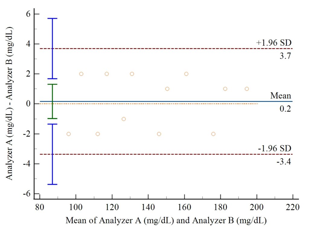
Table-Wise Explanation of Every Result

MedCalc Output	Value	Interpretation	Research Meaning
Method A	Analyzer A	First measurement method	Reference method selected for comparison
Method B	Analyzer B	Second measurement method	Method being evaluated
Sample Size	12	Twelve paired observations analyzed	Each pair contributes one point to the Bland-Altman plot
Plot Option	Plot Differences	Differences plotted against averages	Standard Bland-Altman analysis
Mean Difference (Bias)	0.1667 mg/dL	Very small positive bias	Minimal systematic error between analyzers
95% CI of Bias	−0.9774 to 1.3108	Includes zero	Bias is not statistically different from zero
P-value	0.7545	Greater than 0.05	No significant systematic bias detected
Lower Limit of Agreement	−3.3627 mg/dL	Lowest expected difference	Approximately 95% of differences should remain above this value
95% CI (Lower Limit)	−5.3755 to −1.3498	Precision of lower limit estimate	Wider interval reflects uncertainty from a small sample
Upper Limit of Agreement	3.6960 mg/dL	Highest expected difference	Approximately 95% of differences should remain below this value
95% CI (Upper Limit)	1.6831 to 5.7089	Precision of upper limit estimate	Estimate would become more precise with additional observations

Overall Interpretation

Based on the uploaded MedCalc output, the two analyzers demonstrate minimal average bias (0.1667 mg/dL) and no statistically significant systematic difference (P = 0.7545). The calculated limits of agreement (−3.3627 to 3.6960 mg/dL) describe the range within which most paired differences are expected to fall. These findings indicate good statistical agreement between the two measurement methods. However, the final decision on whether the analyzers can be used interchangeably should be based on whether these limits of agreement are clinically acceptable for the specific analyte and intended application.

Conclusion

The Bland-Altman analysis performed in MedCalc demonstrated a high level of agreement between Analyzer A and Analyzer B. The mean difference (bias) was 0.1667 mg/dL, indicating only a very small systematic difference between the two measurement methods. The 95% confidence interval for the bias included zero, and the P-value (0.7545) confirmed that this difference was not statistically significant.

The calculated 95% limits of agreement, ranging from −3.3627 mg/dL to 3.6960 mg/dL, describe the expected range within which most measurement differences will occur. Visual examination of the Bland-Altman plot showed that the paired differences were randomly scattered around the bias line, with no obvious proportional bias or systematic trend. All observations remained within the calculated limits of agreement, supporting the conclusion that the two methods exhibit good statistical agreement.

Overall, the Bland-Altman method provides a comprehensive assessment of agreement by evaluating both systematic bias and random measurement variability. Compared with correlation analysis, it offers a more appropriate approach for method comparison studies because it directly quantifies measurement differences rather than simply measuring association. Although the present results demonstrate favorable agreement, the ultimate decision regarding the interchangeability of the two analyzers should be based on predefined clinical acceptance criteria, laboratory quality standards, and the specific diagnostic requirements of the analyte being measured.