Introduction
One-way analysis of variance (ANOVA) is commonly used when the objective is to compare the means of a continuous outcome across three or more independent groups. ANOVA answers an important overall question: whether there is evidence that at least one group mean differs from the others. However, a statistically significant ANOVA does not identify which specific groups differ. A post hoc multiple-comparison procedure is therefore useful when the overall test is significant.
The Least Significant Difference (LSD) test is one of the post hoc procedures available in SPSS. It performs pairwise comparisons between group means and reports the mean difference, standard error, significance value, and confidence interval. In this worked example, plant height is compared among a Control group and three supplement groups. The analysis contains four groups with five observations in each group, giving 20 observations in total. The statistical setup used descriptive statistics, a means plot, missing-data analysis, and LSD post hoc testing at the 0.05 significance level.
What Is the LSD Test?
The Least Significant Difference test is a pairwise comparison method used after ANOVA. Its purpose is to determine exactly which group means are significantly different after the omnibus ANOVA has indicated that group differences exist.
Conceptually, the LSD method compares the absolute difference between two sample means with a critical difference based on the within-group error variance and the appropriate degrees of freedom. A simplified expression is:
LSD = t(α/2, error df) × √[MSE(1/nᵢ + 1/nⱼ)]
where MSE is the within-group mean square from ANOVA, nᵢ and nⱼ are the sample sizes for the two groups, and t is the relevant critical value. When the observed mean difference exceeds the LSD threshold, the pair is considered significantly different at the selected alpha level.
Unlike Tukey’s HSD, the classical Fisher LSD procedure does not impose the same strong familywise-error adjustment across all pairwise comparisons. For this reason, LSD is most appropriately used after a significant overall ANOVA and when the comparison plan is scientifically justified. Researchers should report the method clearly rather than treating every post hoc method as interchangeable.
Study Example and Dataset
The dataset contains one response variable, plant height, and one categorical grouping variable with four levels: Control, Supplement A, Supplement B, and Supplement C. Each group contains five replications.
The individual observations are shown below so that the analysis can be reproduced transparently. The group means indicate a clear descriptive pattern. The Control group has the lowest mean plant height (55.84), followed by Supplement A (69.58), Supplement C (71.68), and Supplement B (85.14). These descriptive values agree with the statistical results.
Table 1. Dataset Used for the One-Way ANOVA and LSD Test
| Group | Replication | Plant Height |
|---|---|---|
| Control | 1 | 54.6 |
| Control | 2 | 58.7 |
| Control | 3 | 51.4 |
| Control | 4 | 59.7 |
| Control | 5 | 54.8 |
| Supplement A | 1 | 65.8 |
| Supplement A | 2 | 69.5 |
| Supplement A | 3 | 70.4 |
| Supplement A | 4 | 72.5 |
| Supplement A | 5 | 69.7 |
| Supplement B | 1 | 80.2 |
| Supplement B | 2 | 85.4 |
| Supplement B | 3 | 89.4 |
| Supplement B | 4 | 84.1 |
| Supplement B | 5 | 86.6 |
| Supplement C | 1 | 75.1 |
| Supplement C | 2 | 71.9 |
| Supplement C | 3 | 69.2 |
| Supplement C | 4 | 70.8 |
| Supplement C | 5 | 71.4 |
Concept of One-Way ANOVA Before LSD
Before applying LSD, the one-way ANOVA tests the null hypothesis that all population group means are equal. The alternative hypothesis is that at least one population mean differs.
The ANOVA partitions total variability into between-group variability and within-group variability. For this example, the between-group sum of squares is 2157.348 with 3 degrees of freedom, while the within-group sum of squares is 133.500 with 16 degrees of freedom. The corresponding mean squares are 719.116 and 8.344. The resulting F statistic is 86.186, with the significance value reported in the statistical output as .000. In formal reporting, this should normally be written as p < .001 rather than p = .000.
Because the overall ANOVA is statistically significant, the null hypothesis of equal group means is rejected. The next question is which pairs of groups are responsible for the observed differences. This is where the LSD post hoc analysis becomes useful.
Table 2. One-Way ANOVA Summary for Plant Height
| Source | Sum of Squares | df | Mean Square | F | p-value |
|---|---|---|---|---|---|
| Between Groups | 2157.348 | 3 | 719.116 | 86.186 | < .001 |
| Within Groups | 133.500 | 16 | 8.344 | — | — |
| Total | 2290.848 | 19 | — | — | — |
How to Perform the LSD Test in SPSS
In SPSS, the analysis can be performed through:
Analyze → Compare Means → One-Way ANOVA
Place Plant Height in the Dependent List and Group in the Factor field. Descriptive statistics and a means plot can be selected to summarize the groups visually. Under Post Hoc, select LSD and use a significance level of 0.05.
The analysis specification used for this example included descriptive statistics, a means plot, missing-value analysis, and LSD post hoc comparisons with alpha = 0.05.
The analysis used complete cases for the variables included in the analysis, and the working dataset contained 20 observations.
Interpreting the LSD Pairwise Comparisons
The LSD table shows that Control differs significantly from Supplement A, Supplement B, and Supplement C. The mean differences are −13.74, −29.30, and −15.84, respectively, and all comparisons have p < .001. The negative sign indicates that the Control group has a lower mean plant height than the corresponding supplement group.
Supplement A and Supplement B also differ significantly, with a mean difference of −15.56 and p < .001.
However, Supplement A and Supplement C do not differ significantly. Their mean difference is −2.10, with p = .267. The 95% confidence interval ranges from −5.9728 to 1.7728 and includes zero. Therefore, there is insufficient evidence to conclude that the two groups differ significantly.
Supplement B and Supplement C show a significant difference, with a mean difference of 13.46 and p < .001. The complete pairwise findings are supported by the reported LSD comparisons.
Table 3. Fisher’s LSD Pairwise Comparisons
| Comparison | Mean Difference | SE | p-value | 95% CI Lower | 95% CI Upper | Interpretation |
|---|---|---|---|---|---|---|
| Control vs Supplement A | -13.74 | 1.82688 | < .001 | -17.6128 | -9.8672 | Significant |
| Control vs Supplement B | -29.30 | 1.82688 | < .001 | -33.1728 | -25.4272 | Significant |
| Control vs Supplement C | -15.84 | 1.82688 | < .001 | -19.7128 | -11.9672 | Significant |
| Supplement A vs Supplement B | -15.56 | 1.82688 | < .001 | -19.4328 | -11.6872 | Significant |
| Supplement A vs Supplement C | -2.10 | 1.82688 | .267 | -5.9728 | 1.7728 | Not significant |
| Supplement B vs Supplement C | 13.46 | 1.82688 | < .001 | 9.5872 | 17.3328 | Significant |
Mean Plant Height by Group
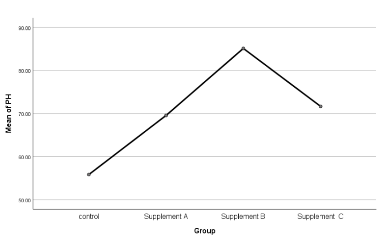
The mean plot demonstrates that the Control group has the lowest average plant height, while Supplement B has the highest average. Supplement A and Supplement C have relatively similar means.
The descriptive means are:
- Control: 55.84
- Supplement A: 69.58
- Supplement B: 85.14
- Supplement C: 71.68
The statistical output reports these group means and their corresponding standard deviations.
The figure therefore provides a useful visual summary of the treatment pattern. The error bars in the accompanying figure represent ±1 standard deviation.
Interpretation of the Mean Plot
The mean plot provides a visual summary of the group differences. Average plant height increases from the Control group to Supplement A, reaches its highest level for Supplement B, and then decreases for Supplement C.
This visual pattern is consistent with the numerical means: 55.84, 69.58, 85.14, and 71.68, respectively.
The plot should be considered a descriptive aid rather than a replacement for inferential testing. In particular, the relatively similar means of Supplement A and Supplement C correspond to their non-significant LSD comparison (p = .267), whereas the larger separation involving Supplement B is supported by statistically significant pairwise comparisons.
How to Report the Result in a Research Article
A concise results statement can be written as follows:
“A one-way ANOVA showed a statistically significant effect of treatment group on plant height, F(3, 16) = 86.186, p < .001. Fisher’s LSD post hoc comparisons showed that the Control group had significantly lower plant height than Supplement A, Supplement B, and Supplement C (all p < .001). Supplement B also produced significantly greater plant height than Supplement A and Supplement C (both p < .001). The difference between Supplement A and Supplement C was not statistically significant (p = .267).”
This reporting style communicates the overall ANOVA result, degrees of freedom, F statistic, significance level, and important pairwise findings. For a thesis or journal article, the result can additionally be presented with mean ± standard deviation for each treatment group.
Key Points to Remember
The LSD test is a post hoc procedure, not a replacement for the overall ANOVA. It is useful for identifying specific group differences after the ANOVA indicates that the group means are not all equal.
The direction of a mean difference should always be interpreted according to the order of the groups in the comparison. A p-value below 0.05 indicates evidence of a statistically significant difference for that particular comparison, whereas a p-value above 0.05 does not provide sufficient evidence of a difference.
Researchers should also consider the assumptions of one-way ANOVA, including independence of observations, approximately normally distributed residuals within groups, and reasonably homogeneous variances. The choice of post hoc procedure should reflect the study design and the desired control of Type I error.
Because Fisher’s LSD is relatively liberal compared with more conservative multiple-comparison procedures, its use should be scientifically justified and clearly reported.
Conclusion
The Least Significant Difference test provides a straightforward method for identifying which specific group means differ after a significant one-way ANOVA.
In this plant-height example, the overall ANOVA was highly significant, F(3, 16) = 86.186, p < .001. The LSD analysis showed significant differences for all comparisons involving the Control group, as well as for Supplement B versus Supplement A and Supplement C. The only non-significant comparison was Supplement A versus Supplement C (p = .267).
Overall, Supplement B had the highest observed mean plant height (85.14), whereas the Control group had the lowest mean (55.84). The results demonstrate how ANOVA and LSD work together: ANOVA establishes that group differences exist overall, while LSD identifies the particular pairs that differ.
When descriptive statistics, an ANOVA table, LSD pairwise comparisons, and a mean plot are presented together, the analysis provides a clear and reproducible interpretation of treatment-related differences in plant height.