Introduction
Autocorrelation Analysis is a statistical technique used to determine whether observations in a dataset are correlated with their own previous values over successive intervals or lags. It is widely applied in time series analysis, ecology, genetics, climatology, economics, engineering, and biological sciences to identify temporal dependence within data.
In PAST (Paleontological Statistics) Statistical Software, autocorrelation analysis is simple to perform and provides both numerical and graphical outputs, making it an excellent tool for students and researchers.
In this tutorial, a sample genetic linkage dataset was analyzed using PAST Statistical Software. The software generated an autocorrelation table and correlogram that help determine whether observations are significantly correlated across different lag values.
What is Autocorrelation?
Autocorrelation, also called serial correlation, measures the relationship between observations separated by a specified number of time steps (lags).
Unlike Pearson correlation, which compares two different variables, autocorrelation compares the same variable with itself after shifting it by one or more observations.
Mathematically,
where
- rk = autocorrelation coefficient at lag k
- Xt = observation at time t
- Xt-k = observation shifted by k lags
Autocorrelation values range between -1 and +1.
- +1 → Perfect positive correlation
- 0 → No correlation
- −1 → Perfect negative correlation
Concept of Lag
A lag represents the number of observations by which the dataset is shifted before computing the correlation.
For example
- Lag 0 → Original data compared with itself
- Lag 1 → Current observation compared with previous observation
- Lag 2 → Compared two observations apart
Increasing lag values help identify repeating patterns and periodicity.
Applications of Autocorrelation
Autocorrelation analysis is widely used in
- Genetics and genomics
- Population biology
- Climate studies
- Environmental monitoring
- Financial forecasting
- Agricultural experiments
- Medical research
- Signal processing
- Ecological monitoring
Sample Dataset
The uploaded dataset consists of 10 generations with measurements from 10 genetic markers (Marker 1–Marker 10). Such datasets can be analyzed to determine whether marker values exhibit serial dependence across generations.
Download Sample Dataset
Autocorrelation Results
The following values were obtained from PAST Statistical Software.
| Lag | Correlation | Confidence Limit |
|---|---|---|
| 0 | 1.00000 | 0.66522 |
| 1 | 0.36299 | 0.71852 |
| 2 | -0.56757 | 0.78710 |
| 3 | -0.78125 | 0.88000 |
| 4 | 0.02774 | 1.01610 |
Interpretation of the Results
| Lag | Interpretation |
|---|---|
| 0 | Correlation equals 1, because every dataset is perfectly correlated with itself. |
| 1 | Weak positive autocorrelation (0.363). The relationship between consecutive observations is relatively small and falls within the confidence limits, indicating no significant serial dependence. |
| 2 | Moderate negative autocorrelation (-0.568). Values two observations apart tend to move in opposite directions, but the correlation is still within the confidence interval and is therefore not statistically significant. |
| 3 | Strong negative autocorrelation (-0.781). Although the coefficient is relatively large in magnitude, it remains inside the confidence bounds, suggesting that the observed negative trend is not statistically significant. |
| 4 | Correlation is close to zero (0.028), indicating virtually no autocorrelation at this lag. |
Interpretation of the Correlogram
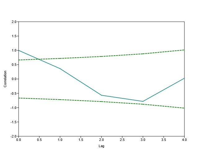
The correlogram provides a graphical representation of autocorrelation across different lag values.
Observations
- The autocorrelation starts at 1.0 for lag 0.
- A gradual decline occurs from lag 0 to lag 3.
- The strongest negative correlation appears at lag 3 (-0.781).
- The correlation returns close to zero at lag 4.
- The dashed confidence limits widen slightly with increasing lag.
- All autocorrelation coefficients remain within the confidence limits.
Overall Interpretation
The analysis indicates that the genetic marker measurements do not exhibit statistically significant autocorrelation across the examined lag values. Although lag 3 shows a relatively strong negative coefficient, it remains within the confidence interval, suggesting that the apparent negative relationship may simply reflect random variation rather than a true serial pattern.
Consequently, the observations can be considered largely independent over the investigated lags.
Discussion
Autocorrelation analysis is particularly valuable when evaluating repeated biological observations. In genetics, detecting significant autocorrelation may indicate inheritance patterns, linkage effects, or temporal dependence among marker measurements.
In this dataset:
- Lag 1 shows only weak positive dependence.
- Lag 2 and lag 3 exhibit negative relationships.
- None of the coefficients exceed the confidence limits.
- Therefore, no statistically meaningful serial dependence is detected.
This suggests that the measured genetic marker values fluctuate independently across generations.
Advantages of Autocorrelation Analysis
- Easy to perform in PAST Software
- Detects hidden temporal dependence
- Identifies cyclic behavior
- Helps validate assumptions of independence
- Useful before regression and forecasting
- Supports biological and ecological research
Limitations
- Small sample sizes reduce statistical power.
- Outliers can influence autocorrelation estimates.
- Only linear relationships are assessed.
- Large lag values are generally less reliable.
- Stationarity assumptions should be considered.
Conclusion
Autocorrelation analysis performed in PAST Statistical Software revealed no statistically significant serial correlation in the sample genetic linkage dataset. Although moderate to strong negative correlations were observed at higher lags, all coefficients remained within their respective confidence limits. The correlogram further confirmed the absence of significant autocorrelation, indicating that the observations are largely independent across generations. Overall, autocorrelation analysis serves as an effective exploratory tool for identifying temporal dependence in biological datasets and should be considered an important preliminary step before conducting advanced time-series or predictive analyses.