Introduction
Multivariate statistical methods are useful when biological or ecological studies contain several variables measured simultaneously. In environmental and biodiversity studies, for example, researchers may measure physicochemical parameters such as pH, temperature, hardness, alkalinity, dissolved oxygen and turbidity, together with the abundance of several species. Analysing these variables separately may not reveal the overall relationship between environmental conditions and biological communities.
Partial Least Squares (PLS) is a multivariate technique that can be used to investigate relationships between two blocks of variables. In ecological studies, one block can contain environmental variables and the second block can contain species abundance or biological variables. PLS reduces these large sets of variables into a smaller number of latent axes while attempting to maximize the covariance between the two blocks.
The PAST statistical software provides a convenient graphical interface for performing Two-block Partial Least Squares analysis. In this tutorial, PLS is demonstrated using a dataset containing 10 sampling sites, 6 environmental variables and 25 species variables.
What is Partial Least Squares (PLS)?
Partial Least Squares (PLS) is a dimensional-reduction and multivariate modelling technique designed to identify relationships between two sets, or blocks, of variables.
In the present analysis:
- Block 1: Environmental variables
- Block 2: Species abundance variables
The environmental block contains:
- pH
- Temperature
- Hardness
- Alkalinity
- Dissolved Oxygen
- Turbidity
The biological block contains Species 1 to Species 25.
Unlike an ordinary correlation analysis, PLS considers multiple variables simultaneously and generates new latent axes. These axes summarize important patterns shared between the two blocks.
Concept of Two-Block PLS
Two-block PLS searches for combinations of variables from the two blocks that have strong covariance.
The basic idea can be represented as:
Environmental variables → PLS axis ← Species variables
Each PLS axis contains:
- Scores – positions of sampling sites on the PLS axis.
- Loadings – contributions of individual variables to the axis.
- Singular values – measures associated with the strength of the extracted axis.
- Percentage covariance – the proportion of covariance represented by each axis.
- Permutation probability – used to assess whether the observed association is stronger than expected by chance.
Therefore, PLS can help answer questions such as:
Which environmental conditions are associated with differences in species composition?
Dataset Used for the PLS Analysis
The supplied dataset contains 10 sampling locations and 31 measured variables in addition to the site identifier.
Table 1. Structure of the dataset
| Component | Variables |
|---|---|
| Sampling sites | 10 |
| Environmental variables | 6 |
| Species variables | 25 |
| Total measured variables | 31 |
| Environmental block | pH, Temperature, Hardness, Alkalinity, Dissolved Oxygen, Turbidity |
| Biological block | Species 1–Species 25 |
The PLS analysis was performed using the Two-block Partial Least Squares option in PAST.
Download Dataset File
How to Perform PLS Analysis in PAST

In PAST, open the dataset and select:
Multivariate → Ordination → Partial Least Squares (PLS)
PAST then opens the Two-block Partial Least Squares analysis window.
The analysis provides several tabs:
- Summary
- Scatter plot
- Scores
- Loadings plot
- Loadings
The analysis can also be calculated using different matrix options, including Correlation and Variance-covariance.
Correlation Matrix PLS Results
The correlation option standardizes the variables and is particularly useful when variables are measured in very different units. This is important for the present dataset because pH, temperature and dissolved oxygen have relatively small numerical values, whereas hardness and turbidity have much larger numerical scales.
Table 2. PLS summary using the correlation matrix
| Axis | Singular value | % Covariance | Permutation p-value |
|---|---|---|---|
| Axis 1 | 2.5117 | 38.4500 | 0.67 |
| Axis 2 | 2.1653 | 28.5750 | 0.14 |
| Axis 3 | 1.6208 | 16.0110 | 0.52 |
| Axis 4 | 1.2654 | 9.7586 | 0.67 |
| Axis 5 | 0.79994 | 3.8999 | 0.84 |
| Axis 6 | 0.73647 | 3.3056 | 0.12 |
The first axis accounts for 38.45% of the covariance, while Axis 2 accounts for 28.575%. Together, the first two axes represent approximately 67.03% of the covariance shown in the PAST summary.
The PAST output reports a squared covariance value of 10.939.
Interpretation
Axis 1 represents the strongest multivariate relationship between the environmental and species blocks. Axis 2 provides the second-largest contribution. Although these axes show the strongest patterns numerically, the permutation probabilities are above 0.05. Therefore, the observed relationships should be regarded as exploratory rather than statistically significant based on the displayed permutation test.
Environmental Loadings
Loadings indicate the contribution and direction of variables along each PLS axis. A positive loading indicates an association in the positive direction of the axis, whereas a negative loading indicates an association in the opposite direction.

Table 3. Environmental-variable loadings for the first two PLS axes
| Environmental variable | Axis 1 | Axis 2 |
|---|---|---|
| pH | 0.5255 | 0.2317 |
| Temperature | -0.1743 | 0.7420 |
| Hardness | -0.0686 | 0.6068 |
| Alkalinity | -0.2832 | 0.1178 |
| Dissolved Oxygen | 0.6591 | 0.0629 |
| Turbidity | 0.4172 | 0.0986 |
Interpretation of Axis 1
Axis 1 is most strongly associated with Dissolved Oxygen (0.6591), followed by pH (0.5255) and Turbidity (0.4172). Alkalinity has a negative loading (-0.2832), while temperature has a relatively weak negative loading (-0.1743).
Thus, the positive direction of Axis 1 is mainly characterized by higher dissolved oxygen, pH and turbidity in the environmental block.
Interpretation of Axis 2
Axis 2 is dominated by Temperature (0.7420) and Hardness (0.6068). The remaining environmental variables have comparatively smaller positive or negative loadings.
Therefore, Axis 2 primarily represents a temperature–hardness gradient within the environmental data.
Species Loadings

The species loadings indicate which species are associated with the environmental gradients represented by each PLS axis.
Table 4. Important species loadings on Axis 1 and Axis 2
| Species | Axis 1 | Axis 2 |
|---|---|---|
| Species 2 | -0.2710 | 0.0026 |
| Species 3 | -0.2367 | -0.0880 |
| Species 4 | 0.3721 | -0.2319 |
| Species 8 | -0.2763 | 0.2639 |
| Species 9 | 0.0817 | 0.3774 |
| Species 12 | -0.0847 | 0.2483 |
| Species 14 | 0.3694 | -0.2082 |
| Species 15 | -0.2956 | -0.1727 |
| Species 21 | -0.3385 | -0.0288 |
| Species 22 | 0.1892 | -0.0361 |
| Species 23 | 0.1184 | -0.3913 |
| Species 24 | 0.1971 | 0.2269 |
| Species 25 | 0.1867 | 0.3319 |
Species with larger absolute loading values contribute more strongly to the corresponding axis.
For Axis 1, Species 21 (-0.3385), Species 4 (0.3721), Species 14 (0.3694), Species 15 (-0.2956) and Species 8 (-0.2763) show relatively strong contributions.
For Axis 2, Species 23 (-0.3913), Species 9 (0.3774), Species 25 (0.3319), Species 8 (0.2639) and Species 12 (0.2483) show relatively stronger contributions.
PLS Scores and Scatter Plot
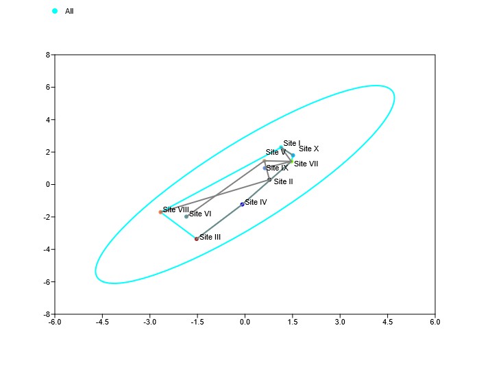
The Scores table gives the position of each sampling site along the PLS axes. The scatter plot provides a visual representation of these scores.
Table 5. PLS scores for the first two axes
| Site | Block 1 Axis 1 | Block 1 Axis 2 | Block 2 Axis 1 | Block 2 Axis 2 |
|---|---|---|---|---|
| Site I | 1.1380 | -0.1098 | 2.2866 | 0.3265 |
| Site II | 0.7712 | 2.2096 | 0.2978 | 3.6170 |
| Site III | -1.5276 | -0.6763 | -3.3607 | -2.2028 |
| Site IV | -0.0856 | -1.2446 | -1.2285 | -3.2808 |
| Site V | 0.6123 | 0.1769 | 1.4591 | 0.8535 |
| Site VI | -1.8492 | 0.1510 | -1.9812 | 0.6490 |
| Site VII | 1.4613 | -0.3390 | 1.4244 | -0.9916 |
| Site VIII | -2.6620 | 1.2746 | -1.7081 | 1.9547 |
| Site IX | 0.6264 | -1.3712 | 1.0090 | 2.1665 |
| Site X | 1.5151 | -0.0712 | 1.7986 | 1.2411 |
The score plot indicates that some sites occupy similar regions of the multivariate space, whereas others are clearly separated.
For example, Site III has strongly negative Axis 1 scores in both blocks, whereas Sites I, VII and X have positive Axis 1 scores. Site II has a particularly high positive Axis 2 score, while Site IV has a strongly negative Axis 2 score.
These patterns suggest differences in environmental conditions and species composition among the sampling locations.
Variance-Covariance PLS Analysis
PAST also provides a variance-covariance option.
Table 6. PLS summary using variance-covariance
| Axis | Singular value | % Covariance | Permutation p-value |
|---|---|---|---|
| Axis 1 | 3647.5 | 98.0810 | 0.81 |
| Axis 2 | 484.6 | 1.7313 | 0.18 |
| Axis 3 | 157.66 | 0.18325 | 0.41 |
| Axis 4 | 23.225 | 0.00397697 | 0.18 |
| Axis 5 | 10.276 | 0.00077847 | 0.11 |
| Axis 6 | 2.5631 | 0.00004843 | 0.18 |
The first axis accounts for approximately 98.08% of the reported covariance. This very strong dominance is largely related to the different numerical scales of the variables.
The squared covariance reported by PAST is 2.9609.
Importantly, the permutation p-value for Axis 1 is 0.81, and Axis 2 is 0.18. Thus, the result does not provide evidence for a statistically significant block relationship at the 0.05 level.
Correlation vs Variance-Covariance: Which is Better?
Table 7. Comparison of the two PLS options
| Feature | Correlation | Variance-Covariance |
|---|---|---|
| Standardization | Yes | No |
| Effect of measurement scale | Reduced | Strong |
| Suitable for different units | Generally better | Less suitable |
| Axis 1 covariance in this analysis | 38.45% | 98.081% |
| Axis 2 covariance | 28.575% | 1.7313% |
| Axis 1 permutation p | 0.67 | 0.81 |
| Main interpretation | More balanced multivariate pattern | Strong scale-driven Axis 1 |
For this dataset, the correlation matrix is generally more informative for exploratory interpretation because the variables are measured on very different scales. The variance-covariance analysis is strongly dominated by the numerical scale of the variables.
Important Data-Quality Observation
One important point should be checked before using these results in a research publication. The supplied Excel dataset contains unusually high values of 82 for Species 2 at Site VI and Species 22 at Site I, while most other species counts are considerably lower.
These values may be genuine observations, but they should be verified against the original field/laboratory records. If 82 is a data-entry error, the PLS analysis should be rerun after correction. If 82 is correct, it should be retained and its ecological relevance considered.
Conclusion
Two-block Partial Least Squares analysis in PAST provides a useful way to examine the multivariate relationship between environmental conditions and species composition. In the present dataset, the correlation-based PLS identified Axis 1 and Axis 2 as the major dimensions, accounting for 38.45% and 28.575% of the reported covariance, respectively.
Environmental loadings showed that dissolved oxygen, pH and turbidity contributed strongly to Axis 1, whereas temperature and hardness were the dominant variables on Axis 2. Several species, including Species 4, Species 14, Species 21, Species 9, Species 23 and Species 25, showed comparatively strong loadings on the first two axes.
The PLS score plot demonstrated differences among sampling sites, with some sites positioned close together and others showing clear separation. However, the permutation probabilities displayed by PAST were greater than 0.05 for the major axes. Therefore, these patterns should be interpreted as exploratory multivariate relationships rather than statistically significant associations.
For this particular dataset, the correlation-based PLS analysis is preferable for interpretation because the environmental variables have substantially different measurement scales. Before final reporting, the unusually high species-abundance values should also be verified.
Overall, PLS in PAST is a valuable ordination-based approach for visualizing and interpreting complex relationships between environmental variables and biological communities.