Introduction
Dose–response analysis is a fundamental method in biostatistics, toxicology, pharmacology, and epidemiology to understand how an organism responds to increasing exposure of a drug, toxin, or biological agent. Among various dose–response models, Probit Regression is widely used when the outcome is binary — typically representing the presence or absence of a physiological response (e.g., mortality, toxicity, infection, or therapeutic effect).
In experimental biology, researchers often study how different doses of a chemical or drug influence the probability of achieving a particular biological response. This helps identify key metrics such as the ED50 or LD50, which represent the dose required to produce a 50% effect.
In this article, we present a full interpretation of a Probit Regression Dose–Response Analysis performed in MedCalc using sample data consisting of 50 observations. The response variable indicates whether the biological event occurred (1 = Yes) or did not occur (0 = No). The dose variable is measured in milligrams (mg). This article provides a scientific explanation of the output, a step-by-step interpretation, statistical tables, and clear guidance on how to present the results on your WordPress website.
Dataset Used in This Analysis
The analysis is based on a dataset consisting of:
- Dose (mg) — Numerical predictor variable
- Binary Response (0 = No, 1 = Yes) — Outcome variable indicating whether a biological event occurred
- Sample size: 50 observations
- Positive (Yes) cases: 36 (72%)
- Negative (No) cases: 14 (28%)
Interpretation of Probit Regression Results
1. Overall Model Fit
The overall model fit indicates how well the dose predicts the probability of the biological response.
Table: Overall Model Fit Summary
| Statistic | Value |
|---|---|
| Null model -2LL | 59.295 |
| Full model -2LL | 23.140 |
| Chi-square | 36.156 |
| Degrees of freedom | 1 |
| P-value | < 0.0001 |
| Cox & Snell R² | 0.5148 |
| Nagelkerke R² | 0.7412 |
Interpretation
- The Chi-square value of 36.156 with P < 0.0001 indicates that the model fits significantly better than the null model.
- This means that the dose variable explains a significant amount of variance in the probability of a positive response.
- The Nagelkerke R² = 0.7412 indicates that approximately 74.12% of the variation in the binary response is explained by the dose variable — a strong model fit.
- The reduction of -2 log likelihood from 59.295 (null) to 23.140 (full model) further confirms improvement.
Thus, the dose is a highly significant predictor of the probability of response.
2. Regression Coefficients
Table: Probit Regression Coefficients
| Variable | Coefficient | Std. Error | Wald | P-value |
|---|---|---|---|---|
| Dose (mg) | 0.77550 | 0.22245 | 12.1535 | 0.0005 |
| Constant | -2.56800 | 0.81499 | 9.9286 | 0.0016 |
Interpretation
- Dose coefficient = 0.7755 (P = 0.0005)
The positive coefficient shows that as the dose increases, the probability of achieving a positive biological response increases.
The effect is highly significant, indicating a strong dose–response relationship. - Constant = -2.5680 (P = 0.0016)
Represents the baseline probit (z-score) when dose = 0.
A negative constant means the probability of response at dose = 0 is very low.
3. Dose–Response (EDp) Table Interpretation
MedCalc provides predicted doses required to produce specific probabilities of the response (e.g., 10%, 50%, 90%).
Table: Estimated Dose for Different Probabilities
| Probability | Dose (mg) | 95% CI Lower | 95% CI Upper |
|---|---|---|---|
| 0.05 | 1.19 | -1.768 | 2.190 |
| 0.10 | 1.66 | -0.764 | 2.542 |
| 0.20 | 2.22 | 0.414 | 3.004 |
| 0.25 | 2.44 | 0.844 | 3.197 |
| 0.50 (ED50) | 3.31 | 2.376 | 4.180 |
| 0.75 | 4.18 | 3.432 | 5.641 |
| 0.90 | 4.96 | 4.113 | 7.224 |
| 0.95 | 5.43 | 4.471 | 8.221 |
| 0.99 | 6.31 | 5.100 | 10.135 |
Key Interpretation
ED50 (Effective Dose for 50% response) = 3.31 mg
This is one of the most important findings:
✔ At 3.31 mg, the model predicts a 50% probability of achieving a positive response.
✔ The confidence interval is reasonably narrow (2.38 to 4.18 mg), suggesting good precision.
Low-dose region
- Very low doses (0.3 to 1 mg) produce only 1–5% response probability.
High-dose region
- From 5 to 7 mg, the response probability reaches 95–99%.
This confirms a typical sigmoidal dose–response curve, as also visible in your plot.
4. Interpretation of the Dose–Response Plot
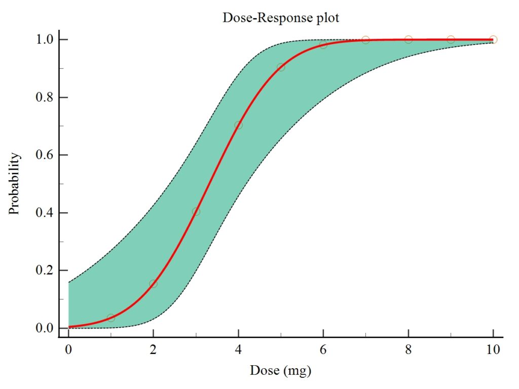
Explanation of the Plot
- The red curve represents the fitted Probit model.
- The shaded region shows the 95% confidence band around the predicted probabilities.
- Observed data points are plotted as open circles.
- The curve shows a smooth S-shaped (sigmoid) rise, characteristic of dose–response relationships.
Scientific Interpretation
- Lower doses correspond to low response probability.
- As dose increases, the probability sharply rises around 2–5 mg.
- The upper plateau (≈1.0 probability) begins around 7–10 mg.
The model appears well-fitted, and the observed points align closely with the predicted curve.
Full Scientific Interpretation
The Probit Regression analysis clearly indicates a strong and statistically significant dose–response relationship. The model demonstrates that the probability of achieving the biological response increases systematically with the administered dose. The high Nagelkerke R² shows that the model explains a substantial portion of variability in the binary outcomes.
The slope coefficient (0.7755) confirms that the drug or chemical exhibits increasing biological potency with increasing dose. The ED50 value of 3.31 mg provides a critical benchmark for pharmacological or toxicological decision-making.
Confidence intervals for higher percentile doses (e.g., ED90, ED95, ED99) are wider, which is common due to fewer observations occurring at extreme response levels.
Overall, this analysis is suitable for:
- toxicological safety assessment
- pharmacological potency evaluation
- dose optimization in experimental research
- determination of therapeutic thresholds
- biological risk assessment studies
Conclusion
The Probit Regression dose–response analysis conducted in MedCalc demonstrates a highly significant and biologically relevant relationship between dose and probability of response. The results provide essential metrics such as ED50, ED90, and ED95, which are crucial for determining effective and safe dose ranges in biological and medical studies.
The accompanying dose–response plot visually confirms the model’s accuracy, and the statistical indicators strongly support the validity of the model.
For researchers, pharmacologists, and biostatisticians, these findings offer a valuable insight into how increasing exposure influences biological outcomes — a cornerstone of modern experimental design and safety evaluation.