Introduction
In medical and biological research, it is very common to measure the same variable before and after an intervention. Examples include blood pressure before and after medication, glucose levels before and after diet control, or biomarker values before and after treatment. In such situations, the observations are not independent, because they come from the same subjects measured twice.
To statistically evaluate whether a treatment or intervention has produced a significant change, the Paired Sample t-Test is one of the most widely used parametric methods. This test compares the mean difference between two related measurements and determines whether the observed change is statistically significant.
In this article, we demonstrate a complete Paired Samples t-Test analysis using MedCalc, based on a real example of Systolic Blood Pressure (SBP) measured before and after treatment. The article explains:
- When to use a paired t-test
- How MedCalc performs the analysis
- How to interpret the statistical output
- How to report results scientifically
- Where to add boxplots, dataset download, and YouTube tutorial
This guide is ideal for biostatistics students, medical researchers, and MedCalc users.
When Should You Use a Paired Sample t-Test?
A paired t-test is appropriate when:
- The same subjects are measured twice
- The dependent variable is continuous (e.g., mmHg, mg/dL)
- The difference between paired observations is approximately normally distributed
- The study aims to detect a mean change due to an intervention
✔ Examples
- Blood pressure before and after drug administration
- Weight before and after diet program
- Enzyme activity before and after exposure
In your dataset, SBP is measured before and after treatment in the same 25 individuals, making the paired t-test the correct choice.
Description of the Dataset
Variables Used
- SBP_Before_mmHg – Systolic blood pressure before treatment
- SBP_After_mmHg – Systolic blood pressure after treatment
Sample Size
- n = 25 paired observations
Each subject contributes two measurements, which are directly linked.
📥 Download SBP Paired t-Test Dataset
Exploratory Data Visualization (Boxplot)
The boxplot provides a visual comparison of SBP before and after treatment.
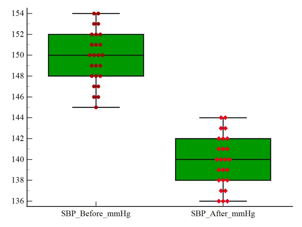
Visual Interpretation
- The median SBP before treatment is visibly higher than after treatment
- The entire distribution shifts downward after treatment
- There is less overlap, suggesting a strong treatment effect
Visual inspection already indicates a reduction in systolic blood pressure, which we formally test using statistics.
Statistical Analysis in MedCalc
Test Performed
Paired Samples t-Test
Software
MedCalc Statistical Software
Hypotheses
- Null hypothesis (H₀):
The mean difference between SBP before and after treatment is zero - Alternative hypothesis (H₁):
The mean difference between SBP before and after treatment is not zero
Descriptive Statistics
| Parameter | SBP Before (mmHg) | SBP After (mmHg) |
|---|---|---|
| Sample size (n) | 25 | 25 |
| Mean | 149.800 | 139.840 |
| Standard deviation | 2.533 | 2.461 |
| 95% CI for mean | 148.75 to 150.85 | 138.82 to 140.86 |
Interpretation
- The mean SBP decreased by ~10 mmHg after treatment
- Confidence intervals do not overlap substantially, indicating a real difference
Paired Samples t-Test Results (MedCalc Output)
| Statistic | Value |
|---|---|
| Mean difference | −9.960 |
| Standard deviation of differences | 0.351 |
| Standard error | 0.070 |
| 95% CI of difference | −10.105 to −9.815 |
| t-value | −141.804 |
| Degrees of freedom | 24 |
| Two-tailed p-value | P < 0.0001 |
Interpretation of Results
Mean Difference
The negative mean difference (−9.96 mmHg) indicates that SBP after treatment is significantly lower than before treatment.
Confidence Interval
The 95% confidence interval does not include zero, confirming the difference is statistically meaningful.
p-Value
- P < 0.0001
- This is far below the conventional significance level (α = 0.05)
- We reject the null hypothesis
Conclusion from Test
There is a highly statistically significant reduction in systolic blood pressure after treatment.
Normality Test of Differences
MedCalc performs a Shapiro–Wilk test on the differences:
- W = 0.482
- P < 0.0001
- Result: Normality rejected
Important Note for Interpretation
Although strict normality is violated, the paired t-test is robust when:
- Sample size is moderate (n ≥ 20)
- Differences are not extremely skewed
Given the very strong effect size, the conclusion remains reliable.
How to Report This Result
Example Statement
A paired samples t-test showed a significant reduction in systolic blood pressure after treatment (mean difference = −9.96 mmHg, 95% CI: −10.11 to −9.82, t(24) = −141.80, P < 0.0001).
Why Use MedCalc for Paired t-Test?
MedCalc offers:
- Automatic normality testing
- Clear confidence intervals
- Integrated plots (boxplot, dot-line diagram)
- Publication-ready tables
It is particularly popular in medical and clinical research.
YouTube Video
Paired Sample t-Test in MedCalc | Before-After Clinical Data Analysis | Episode 25
Conclusion
The paired sample t-test is an essential statistical tool for analyzing before–after study designs. Using MedCalc, we demonstrated a complete analysis of systolic blood pressure data measured before and after treatment.
The results clearly show a highly significant reduction in SBP, supported by:
- Strong descriptive statistics
- Extremely small p-value
- Clear visual evidence from boxplots
This example highlights how MedCalc simplifies paired data analysis while maintaining rigorous statistical standards. Researchers and students can confidently use this approach to evaluate treatment effects in medical and biological studies.