Introduction
Cluster analysis is an important multivariate statistical technique used to classify observations into groups according to their similarity. Unlike many conventional statistical methods, cluster analysis does not require predefined group labels. Instead, the method searches for naturally occurring patterns within a dataset and assigns observations to groups called clusters.
K-means clustering is one of the most widely used partitioning methods. It is particularly useful when researchers want to explore whether observations can be separated into a specified number of relatively similar groups. In biological and ecological research, it can be applied to species abundance, environmental measurements, morphological characteristics, sampling sites, community composition and other multivariable datasets.
The PAST (Paleontological Statistics) software provides an accessible environment for performing K-means clustering and examining cluster membership and silhouette values. In this example, 15 butterfly species were evaluated using observations from 10 sites. The analysis was performed with two clusters (k = 2).
The objective was to determine whether the butterfly species could be separated into two groups based on their patterns across the ten sampling sites.
What is Cluster Analysis?
Cluster analysis is an exploratory multivariate technique that groups observations according to their similarity or dissimilarity.
For example, suppose several butterfly species have abundance values recorded at different sampling sites. Species showing similar distribution patterns across the sites may be placed in the same cluster.
The important point is that cluster analysis is generally unsupervised. The researcher does not initially tell the method which species belong together. Instead, the algorithm identifies groupings from the supplied numerical variables.
Basic concept
The process can be represented as:
Raw multivariate data
↓
Calculate similarity/distance
↓
Select number of clusters
↓
Assign observations to clusters
↓
Calculate cluster centres
↓
Evaluate cluster separation
↓
Interpret biological/ecological patterns
What is K-Means Clustering?
K-means clustering is a partitioning algorithm that divides observations into a predefined number of clusters, represented by K.
In this analysis:
K = 2
Therefore, the 15 butterfly species were divided into two clusters.
The algorithm attempts to place observations into clusters so that observations within the same cluster are relatively similar, while observations belonging to different clusters are relatively different.
Conceptually, K-means minimizes the within-cluster sum of squares (WGSS):
where:
- = number of clusters
- = observations belonging to cluster
- = individual observation
- = centroid of cluster
- = distance between an observation and its cluster centroid
The algorithm repeatedly updates the cluster assignments and cluster centres until the grouping stabilizes.
Dataset Used for the Analysis
The uploaded dataset contains 15 butterfly species and measurements from 10 sites.
Table 1. Structure of the dataset
| Variable | Description |
|---|---|
| Butterfly Species | Observation/species identifier |
| Site 1 | Observation at Site 1 |
| Site 2 | Observation at Site 2 |
| Site 3 | Observation at Site 3 |
| Site 4 | Observation at Site 4 |
| Site 5 | Observation at Site 5 |
| Site 6 | Observation at Site 6 |
| Site 7 | Observation at Site 7 |
| Site 8 | Observation at Site 8 |
| Site 9 | Observation at Site 9 |
| Site 10 | Observation at Site 10 |
| Number of species | 15 |
| Number of numerical variables | 10 |
The species names were represented as Species A through Species O.
Download Dataset
K-Means Analysis in PAST
The K-means analysis was performed using two clusters.
The resulting PAST output showed:
| PAST output | Result |
|---|---|
| Number of clusters | 2 |
| WGSS | 2172.9 |
| F | 0.32397 |
| Var % | 24.47 |
| Average silhouette | 0.027853 |
The WGSS (within-group sum of squares) represents the total within-cluster variation associated with the solution. Lower within-cluster variation generally corresponds to more compact clusters, although WGSS should not be interpreted independently of the number of clusters.
The average silhouette value provides information about how well observations fit their assigned clusters. Values close to 1 indicate strong separation, values around zero indicate substantial overlap or observations near cluster boundaries, and negative values indicate observations that may be closer to another cluster than their assigned cluster.
K-Means Cluster Membership
The PAST analysis divided the 15 butterfly species into two groups.
Table 2. K-means cluster membership of butterfly species
| Cluster | Butterfly species | Number of species |
|---|---|---|
| Cluster 1 | Species A, C, E, F, I, L, N, O | 8 |
| Cluster 2 | Species B, D, G, H, J, K, M | 7 |
Thus, Cluster 1 contained eight species, whereas Cluster 2 contained seven species.
Cluster 1
Species A, C, E, F, I, L, N and O.
Cluster 2
Species B, D, G, H, J, K and M.
The cluster numbers themselves are labels rather than biological categories. Therefore, Cluster 1 should not automatically be interpreted as a “high” or “low” group without examining the underlying variables.
Silhouette Analysis
The silhouette table provides an observation-level assessment of the clustering solution.
Table 3. Silhouette values for the two-cluster solution
| Species | Cluster | Silhouette |
|---|---|---|
| Species F | 1 | 0.117710 |
| Species N | 1 | 0.110850 |
| Species I | 1 | 0.096642 |
| Species C | 1 | 0.086835 |
| Species O | 1 | 0.038808 |
| Species E | 1 | 0.038424 |
| Species L | 1 | -0.033244 |
| Species A | 1 | -0.174240 |
| Species H | 2 | 0.208510 |
| Species M | 2 | 0.132470 |
| Species D | 2 | 0.109140 |
| Species B | 2 | 0.048865 |
| Species J | 2 | -0.060232 |
| Species K | 2 | -0.090194 |
| Species G | 2 | -0.212550 |
The overall mean silhouette calculated from the displayed individual values is approximately 0.02785, matching the PAST output.
Interpretation of Silhouette Results
The silhouette results provide an important qualification to the cluster membership.
Several species have positive silhouette values, indicating some degree of association with their assigned cluster. For example, Species H has the highest silhouette value in the displayed output at 0.208510, followed by Species M (0.132470), Species F (0.117710), Species N (0.110850) and Species D (0.109140).
However, the overall average silhouette is only 0.027853. This is close to zero, indicating that the two clusters have considerable overlap in multivariate space.
Several species also have negative silhouette values:
- Species A = -0.174240
- Species G = -0.212550
- Species K = -0.090194
- Species J = -0.060232
- Species L = -0.033244
A negative silhouette value does not mean that the species is biologically incorrect or that the analysis has failed. Rather, it indicates that the observation is relatively close to the alternative cluster according to the distance structure used in the analysis.
Therefore, the K-means result should be regarded as an exploratory grouping, rather than definitive evidence that the butterfly species form two strongly separated groups.
Cluster Characteristics
The mean values for each site can also help describe the two clusters.
Table 4. Mean site values by cluster
| Site | Cluster 1 Mean | Cluster 2 Mean |
|---|---|---|
| Site 1 | 8.875 | 8.857 |
| Site 2 | 10.250 | 7.571 |
| Site 3 | 7.375 | 13.000 |
| Site 4 | 11.250 | 8.571 |
| Site 5 | 10.000 | 12.000 |
| Site 6 | 12.000 | 8.000 |
| Site 7 | 12.375 | 8.429 |
| Site 8 | 6.250 | 14.286 |
| Site 9 | 14.000 | 8.286 |
| Site 10 | 8.875 | 12.000 |
The cluster means show that the two groups have different patterns across several sites.
Cluster 1 has higher mean values at Sites 2, 4, 6, 7 and 9, while Cluster 2 has higher mean values at Sites 3, 5, 8 and 10. Site 1 has almost identical means between the two clusters.
This suggests that the clustering is driven by different distribution patterns across sampling sites, rather than by a simple overall difference in abundance.
K-Means Cluster Pattern
The supplied horizontal bar plot illustrates the relative positioning of the butterfly species associated with the two-cluster solution.
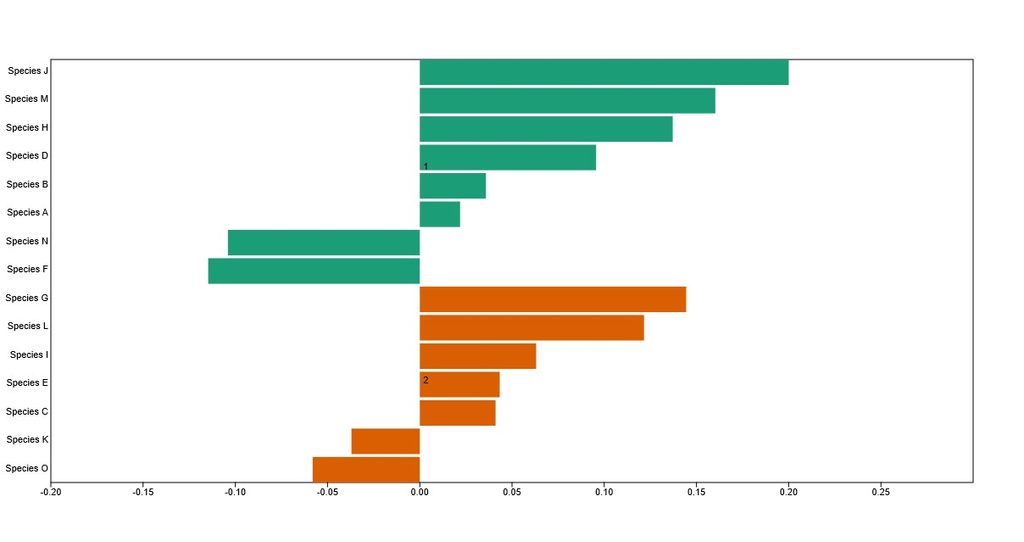
Figure 1. K-means clustering pattern of the 15 butterfly species based on observations across 10 sites.
The figure can be interpreted together with the cluster membership table. Species positioned relatively close to one another according to the underlying multivariate measurements show greater similarity, whereas species separated from one another represent greater dissimilarity.
The visual pattern should not be interpreted as a direct measure of statistical significance. Rather, it provides a graphical representation of the multivariate relationships identified by the analysis.
Biological Interpretation
The K-means analysis indicates that the butterfly species can be partitioned into two groups based on their recorded patterns across the ten sites.
Cluster 1 consists of Species A, C, E, F, I, L, N and O. This group shows relatively higher average values at several sites, particularly Sites 6, 7 and 9.
Cluster 2 consists of Species B, D, G, H, J, K and M. This group shows comparatively higher averages at Sites 3, 5, 8 and 10.
These differences may indicate that the two groups have different spatial distribution patterns in the study dataset. However, the cluster analysis alone cannot establish the ecological mechanism responsible for these patterns. Environmental variables, habitat characteristics, season, resource availability and other ecological factors would need to be examined separately before making biological explanations.
The low average silhouette value is particularly important. It indicates that the species are not separated into two highly distinct groups based on the variables included in the analysis.
Important Point About the Number of Clusters
K-means requires the researcher to specify the number of clusters in advance. Here, K = 2 was selected.
However, choosing two clusters does not automatically mean that two clusters provide the only or optimal representation of the dataset.
A researcher can compare solutions using:
- K = 2
- K = 3
- K = 4
- K = 5
and examine measures such as:
- Within-group sum of squares
- Silhouette values
- Cluster stability
- Biological interpretability
- Separation between clusters
For this dataset, the low average silhouette for K = 2 suggests that examining alternative cluster numbers could be useful before drawing strong conclusions.
Limitations of K-Means Clustering
K-means also has important limitations.
First, the number of clusters must be specified before the analysis. Second, the method can be affected by the scale of variables. If variables are measured on very different scales, standardization may be necessary.
The method can also be sensitive to the starting positions of cluster centres and to unusual observations. Furthermore, K-means works best when the underlying groups are reasonably compact and distinguishable using the selected distance measure.
Therefore, cluster membership should not automatically be interpreted as a biological classification. It is a statistical grouping based on the variables supplied to the analysis.
Results Summary
Table 5. Summary of K-means clustering results
| Parameter | Result |
|---|---|
| Observations | 15 species |
| Numerical variables | 10 sites |
| Number of clusters | 2 |
| Cluster 1 | 8 species |
| Cluster 2 | 7 species |
| WGSS | 2172.9 |
| F | 0.32397 |
| Variance (%) | 24.47 |
| Average silhouette | 0.027853 |
Main finding
The K-means procedure divided the 15 butterfly species into two groups:
Cluster 1: A, C, E, F, I, L, N and O
Cluster 2: B, D, G, H, J, K and M
The average silhouette value of 0.027853 indicates that the two groups show substantial overlap and that the separation between clusters is weak in this particular two-cluster solution.
Conclusion
K-means cluster analysis provides a useful exploratory approach for identifying groups of similar observations in multivariate biological datasets. In the present analysis, 15 butterfly species characterized by observations from 10 sites were classified into two clusters using PAST.
Cluster 1 contained eight species—A, C, E, F, I, L, N and O—whereas Cluster 2 contained seven species—B, D, G, H, J, K and M. The cluster means demonstrated different patterns across the ten sampling sites, suggesting that the groups differ in their distribution profiles.
However, the average silhouette value of 0.027853, together with several negative individual silhouette values, indicates substantial overlap between the two groups. Consequently, the current K = 2 solution should be interpreted as an exploratory pattern rather than a strongly separated classification.
For a more robust analysis, researchers may compare different numbers of clusters and examine silhouette values and biological interpretability before selecting a final clustering solution. Combining K-means results with ecological information and appropriate visualization can provide a more complete understanding of species distribution patterns.