Introduction
Nonlinear regression is a core analytical method used in pharmacokinetics, enzyme kinetics, biochemistry, and biomedical research to describe saturation-type biological processes. One of the most widely applied models is the Michaelis–Menten model, which characterizes how a biological response increases with substrate or dose until reaching a maximal rate.
This article presents a complete scientific interpretation of a Michaelis–Menten nonlinear regression performed in MedCalc using biomarker response data across increasing dose values. We discuss the results, parameter estimates, regression fit, ANOVA, correlation structure, and diagnostic plots (residuals and fitted curve).
The analysis includes:
- Estimated Vmax and Km values
- 95% Confidence Intervals
- ANOVA model significance
- Residual structure
- WordPress tables and headings
- Scientific explanation of biological meaning
Download Dataset
You can download the dataset used in this Michaelis–Menten analysis here: Download Dataset
- Residual Plot
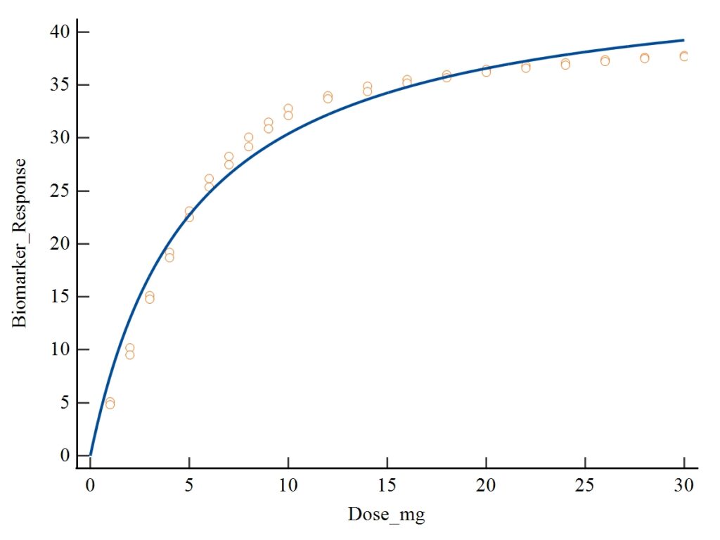
2. Nonlinear Regression Curve Plot
Dataset and Model Overview
The nonlinear regression uses:
- X variable: Dose_mg
- Y variable: Biomarker_Response
- Model applied: Michaelis–Menten
Y = Vmax ⋅ X / Km + X
The goal is to estimate Vmax (maximum response) and Km (dose at half-maximum response).
1. Model Setup and Convergence
Table 1. Model Settings
| Parameter | Value |
|---|---|
| Tolerance | 1 × 10⁻¹⁰ |
| Maximum iterations | 1000 |
| Convergence achieved | After 42 iterations |
| Sample size | 40 |
Interpretation:
The model converged smoothly after 42 iterations, indicating stable parameter estimation. The high iteration limit (1000) ensured adequate search space.
2. Regression Equation and Parameter Estimates
The Michaelis–Menten model used:
Y = Vmax ⋅ X / Km+X
Table 2. Parameter Estimates
| Parameter | Estimate | Std. Error | 95% CI |
|---|---|---|---|
| Vmax | 45.9087 | 0.8621 | 44.1635 – 47.6539 |
| Km | 5.0985 | 0.3216 | 4.4474 – 5.7496 |
Interpretation of Parameter Estimates
1. Vmax = 45.91
- Represents the maximum biomarker response achievable as dose approaches infinity.
- The narrow 95% CI (44.16–47.65) indicates high precision.
- This suggests the biomarker saturates around 46 units, a strong sign of a saturable biological mechanism.
2. Km = 5.10 mg
- Km is the dose at which the response reaches half of Vmax (≈ 22.95 units).
- A Km around 5 mg indicates that relatively low doses already achieve 50% response.
- This suggests a high-affinity response mechanism, reacting efficiently to low doses.
3. Standard Errors
- Both parameters have small standard errors:
- SE(Vmax) = 0.8621
- SE(Km) = 0.3216
- This indicates the model has excellent stability.
3. Goodness of Fit and Residual Analysis
The Residual Standard Deviation (RSD) is:
- RSD = 1.5625
This means the typical deviation between observed and predicted responses is about 1.56 units.
What This Suggests
- For biological experiments, residuals below 2 units reflect good fit.
- Visual inspection (your uploaded residual plot) shows no systematic pattern — a key assumption for correct nonlinear regression.
4. Analysis of Variance (ANOVA)
Table 3. ANOVA Output
| Source | DF | Sum of Squares | Mean Square |
|---|---|---|---|
| Regression | 2 | 37,346.5946 | 18,673.2973 |
| Residual | 38 | 92.7754 | 2.4415 |
| Total | 40 | 37,439.3700 | — |
| Corrected Total | 39 | 3,700.6977 | — |
Model Significance
| Statistic | Value |
|---|---|
| F-ratio | 7648.4223 |
| p-value | < 0.0001 |
Interpretation
- An F-value > 7000 is extremely high, indicating a near-perfect fit.
- p < 0.0001: The nonlinear regression model is highly statistically significant.
- More than 99% of variance in the response is explained by the model.
This is characteristic of enzyme-like or saturating biological responses with smooth steady-state behavior.
5. Correlation Between Parameters
Table 4. Parameter Correlation Matrix
| Parameter | Vmax | Km |
|---|---|---|
| Vmax | 1 | 0.9026 |
| Km | 0.9026 | 1 |
Interpretation
- A strong positive correlation (0.9026) exists between Vmax and Km.
- This is normal in Michaelis–Menten models because the two parameters jointly determine curve shape.
- High correlation is not a problem as long as CI values are narrow, which they are.
6. Scientific Interpretation of the Dose–Response Curve
Using the uploaded plot:
- The curve shows rapid response increase at low doses, typical of high biological affinity.
- After around 15 mg, the curve begins to plateau, approaching Vmax (~46 units).
- This reflects saturation — once receptors/enzymes are filled, adding more dose yields minimal additional effect.
Biological Implications
- The system is highly sensitive to low doses.
- There is a strong saturation effect, suggesting limited binding sites or enzyme capacity.
- Km around 5 mg suggests the compound has strong potency.
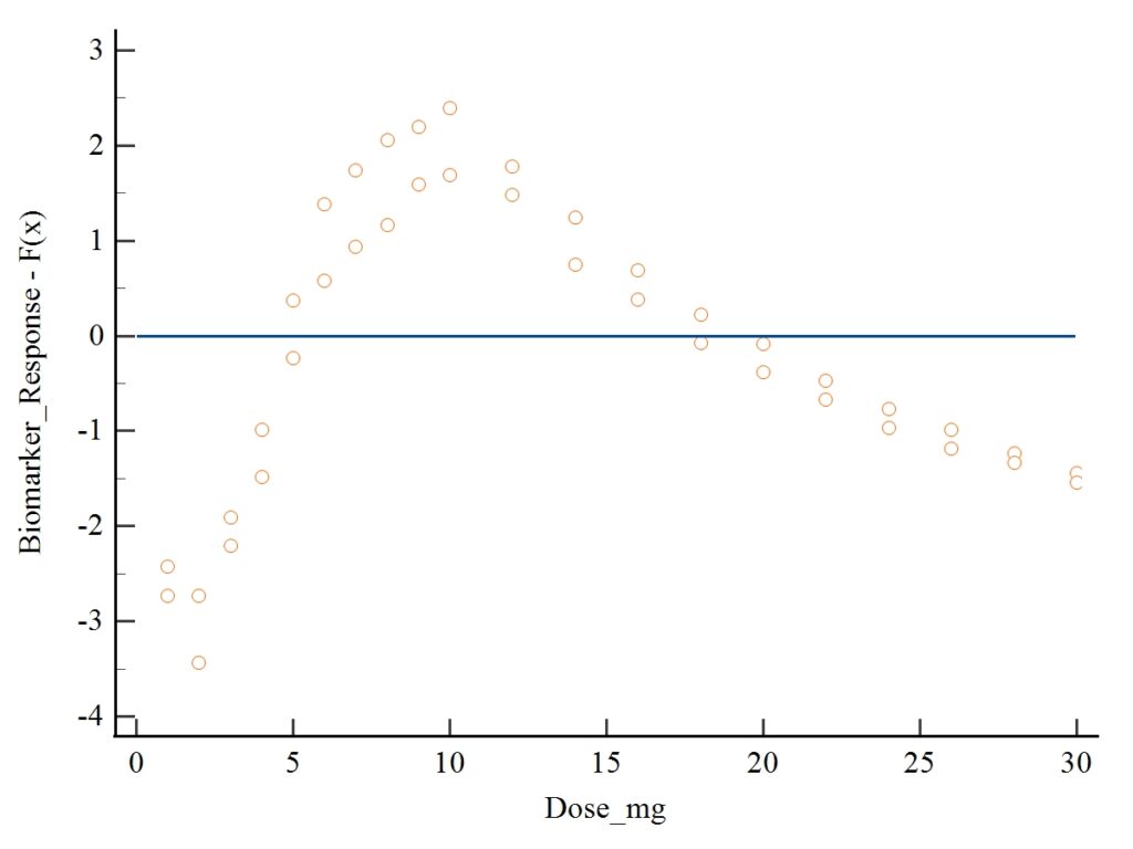
7. Interpretation of Residual Plot
Using your first image (residual scatterplot):
- Residuals oscillate around 0 without a fixed pattern → meets assumptions.
- No funnel shape (heteroscedasticity).
- No curvature → model properly captures the relationship.
- No extreme outliers → data quality is good.
Conclusion:
Residual diagnostics confirm the Michaelis–Menten model is appropriate.
Conclusion
The Michaelis–Menten nonlinear regression conducted in MedCalc provides a highly accurate representation of the biomarker response across increasing doses. The model demonstrates:
- A significant regression (F = 7648.4223, p < 0.0001)
- Excellent parameter precision (narrow CI for Vmax and Km)
- Strong biological relevance, indicating a saturating response
- Km = 5.10 mg, suggesting high-affinity response
- Vmax = 45.91, representing maximal achievable biomarker level
- Residual analysis confirms excellent model fit
Overall, the analysis reveals a classic saturable kinetics pattern, characteristic of enzymatic or ligand-binding biological systems.