Introduction

In biomedical and clinical research, measurements are often collected repeatedly from the same patient over time. Examples include blood glucose levels, blood pressure readings, tumor size measurements, cholesterol levels, and biomarker concentrations recorded during follow-up visits.

Analyzing such repeated observations requires specialized statistical methods because the measurements are not independent. MedCalc provides a dedicated Serial Measurements module that summarizes repeated observations into meaningful metrics and compares these values among groups.

This tutorial explains the complete workflow of Serial Measurements Analysis in MedCalc, including data preparation, option settings, Area Under the Curve (AUC) calculation, statistical testing, interpretation of results, and graphical visualization.

What is Serial Measurements Analysis?

Serial Measurements Analysis is a statistical approach used to evaluate changes in a variable measured repeatedly over time in the same subject.

Instead of analyzing every time point separately, MedCalc can summarize the entire response profile using measures such as:

• Minimum value
• Maximum value
• First observation
• Last observation
• Difference between observations
• Time-weighted average
• Area Under the Curve (AUC)
• Percentage time above or below a threshold

This approach provides a single summary value for each subject, making group comparisons easier.

Why Use Serial Measurements Analysis?

Serial measurements are common in:

Clinical Trials

• Drug efficacy studies
• Vaccine response studies
• Diabetes monitoring

Biomedical Research

• Biomarker tracking
• Disease progression studies

Pharmacology

• Drug concentration monitoring
• Pharmacokinetic studies

Epidemiology

• Long-term health monitoring

Example Dataset

The following glucose measurements were recorded at four different follow-up visits.

Patient_ID	Group	Week	Glucose
P1	Drug A	0	180
P1	Drug A	4	160
P1	Drug A	8	145
P1	Drug A	12	130
P2	Drug B	0	190
P2	Drug B	4	170
P2	Drug B	8	150
P2	Drug B	12	135
P3	Placebo	0	195
P3	Placebo	4	205
P3	Placebo	8	190
P3	Placebo	12	215

Understanding the Trend

Drug A

Glucose continuously decreases from 180 to 130.

Drug B

Glucose continuously decreases from 190 to 135.

Placebo

Glucose remains high and eventually increases.

This suggests that Drug A and Drug B improve glucose control compared with placebo.

Step-by-Step Procedure in MedCalc

Step 1: Import Data

Open MedCalc and enter the dataset with columns:

• Patient_ID
• Group
• Week
• Glucose

Step 2: Open Serial Measurements

Navigate to:

Statistics → Longitudinal Data → Serial Measurements

The Serial Measurements dialog box appears.

Step 3: Assign Variables

Variable Y (data)

Select:

Glucose

Variable X (time)

Select:

Week

Cases Identification

Select:

Patient_ID

Groups

Select:

Group

Explanation of Summary Measure Options

MedCalc provides several summary measures.

Minimum

Smallest observed value.

Example:
Lowest glucose level recorded.

Maximum

Largest observed value.

Example:
Highest glucose level recorded.

First Observation

Value at baseline.

Example:
Week 0 glucose.

Last Observation

Final recorded value.

Example:
Week 12 glucose.

Difference Last-First

$$Last – First$$

Shows overall change during follow-up.

Max Difference vs First

$$Maximum – First$$

Measures largest increase relative to baseline.

Time-Weighted Average

Accounts for both value and duration.

Useful when intervals between measurements differ.

Area Under Curve (AUC)

Selected in this analysis.

AUC summarizes the entire response profile over time.

Higher AUC indicates greater overall exposure to the measured variable.

% Time Above Threshold

Calculates percentage of time above a specified value.

Example:
Percentage of time glucose remains above 180 mg/dL.

% Time Below Threshold

Calculates percentage of time below a threshold.

Selected Settings Used in This Analysis

Summary Measure

✔ Area Under Curve (Baseline = 0)

Statistical Analysis

✔ Automatic

Test for Normal Distribution

✔ D’Agostino-Pearson Test

Groups

✔ Drug A
✔ Drug B
✔ Placebo

Why AUC Was Selected

AUC incorporates:

• Magnitude of glucose values
• Duration of exposure
• Entire follow-up period

Rather than focusing on one time point, AUC evaluates the overall treatment response.

Baseline Options Explained

Baseline = 0

Area calculated relative to zero.

Used in your analysis.

Baseline = First Value

Area calculated relative to baseline measurement.

Useful when assessing treatment effect relative to starting value.

Baseline = Minimum

Area calculated relative to the lowest observed value.

Useful in some pharmacological studies.

Statistical Analysis Options

Automatic

MedCalc automatically selects the appropriate statistical test.

Parametric Test

Used when data follow normal distribution.

Examples:

• t-test
• ANOVA

Non-Parametric Test

Used when normality assumptions are violated.

Examples:

• Mann–Whitney test
• Kruskal–Wallis test

Parametric Test After Log Transformation

Used for skewed data that become normal after logarithmic transformation.

Normality Test Options

Shapiro-Wilk Test

Best for small sample sizes.

Shapiro-Francia Test

Alternative normality test.

D’Agostino-Pearson Test

Combines skewness and kurtosis.

Kolmogorov-Smirnov Test

Compares sample distribution with theoretical distribution.

Results Obtained

Area Under Curve (AUC)

Group	AUC
Drug A	1840
Drug B	1930
Placebo	2400

Interpretation of AUC

Drug A

AUC = 1840

Lowest AUC value.

Indicates best glucose control.

Drug B

AUC = 1930

Slightly higher than Drug A.

Still demonstrates effective glucose reduction.

Placebo

AUC = 2400

Highest AUC value.

Shows poor glucose control.

Ranking of Treatments

Rank	Group	Performance
1	Drug A	Best
2	Drug B	Good
3	Placebo	Poor

Kruskal-Wallis Test Results

Statistic	Value
Test Statistic	2.000
Degrees of Freedom	2
P-value	0.3679

Interpretation

Since:$$P = 0.3679 > 0.05$$P=0.3679>0.05

there is no statistically significant difference among the groups.

Why No Significant Difference?

The dataset contains:

• Only 1 subject per group
• Very small sample size

With larger sample sizes, significant differences would be more likely to appear.

Graph Interpretation

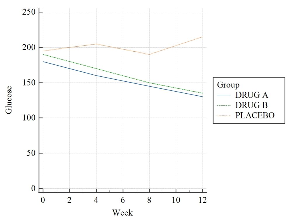
Glucose vs Week Plot

Drug A

Steady decrease in glucose levels.

Drug B

Steady decrease in glucose levels.

Placebo

No improvement.

This visual pattern supports the AUC findings.

Clinical Interpretation

The analysis suggests:

• Drug A provides the strongest glucose reduction.
• Drug B also improves glucose control.
• Placebo fails to control glucose effectively.
• Larger studies are required to confirm significance.

Advantages of Serial Measurements Analysis

✔ Uses entire follow-up period

✔ Reduces repeated testing issues

✔ Summarizes longitudinal data efficiently

✔ Useful in clinical trials

✔ Supports AUC calculations

✔ Allows group comparison

✔ Easy interpretation

Conclusion

Serial Measurements Analysis in MedCalc is a powerful tool for analyzing longitudinal biomedical data. By summarizing repeated observations into meaningful metrics such as Area Under the Curve (AUC), researchers can evaluate treatment effects more efficiently. In this glucose monitoring example, Drug A achieved the lowest AUC and demonstrated the best glucose control, while Placebo showed the poorest performance. Although the small sample size resulted in a non-significant Kruskal-Wallis test, the methodology illustrates how MedCalc can be used to analyze repeated measurements in clinical and biomedical research effectively.