Introduction
Meta-analysis is a powerful statistical technique used to combine the results of multiple independent studies into a single summary estimate. Researchers often encounter situations where published studies report effect estimates and standard errors rather than raw data. In such cases, the Generic Inverse Variance (GIV) Method becomes extremely useful.
The Generic Inverse Variance Method allows researchers to combine effect estimates such as regression coefficients, log odds ratios, log risk ratios, hazard ratios, and other summary statistics using their standard errors. MedCalc provides a simple and user-friendly environment for performing this analysis.
In this tutorial, we will learn how to perform a Meta-Analysis using the Generic Inverse Variance Method in MedCalc, understand its underlying concepts, interpret outputs, and explain forest plots and funnel plots using a practical example.
What is the Generic Inverse Variance Method?
The Generic Inverse Variance Method is a meta-analysis technique where each study contributes an effect estimate and its standard error.
The weight assigned to each study is:
Where:
- SE = Standard Error of the study estimate
Studies with smaller standard errors receive larger weights because they provide more precise information.
Why Use the Generic Inverse Variance Method?
This method is useful when:
✓ Raw event data are unavailable
✓ Published studies report effect estimates only
✓ Combining adjusted estimates from regression models
✓ Combining hazard ratios from survival analysis
✓ Combining odds ratios and risk ratios after log transformation
✓ Combining beta coefficients from observational studies
Data Used in This Example
The following variables were entered into MedCalc:
| Study | Estimate | Standard Error |
|---|---|---|
| Study 1 | 0.820 | 0.120 |
| Study 2 | 0.750 | 0.100 |
| Study 3 | 0.880 | 0.090 |
| Study 4 | 0.790 | 0.110 |
| Study 5 | 0.720 | 0.080 |
| Study 6 | 0.850 | 0.100 |
| Study 7 | 0.770 | 0.090 |
| Study 8 | 0.810 | 0.110 |
The analysis combines these study estimates into a single pooled estimate.
Step-by-Step Procedure in MedCalc
Step 1: Prepare Data
Create three columns:
| Column | Description |
|---|---|
| Study | Study Name |
| Estimate | Effect Size |
| Standard Error | Standard Error of Estimate |
Enter the data for all studies.
Step 2: Open Meta-Analysis
Navigate to:
Statistics → Meta-analysis → Generic Inverse Variance Method
Step 3: Select Variables
Assign:
- Study Variable = Study
- Estimate Variable = Estimate
- Standard Error Variable = Standard Error
Click OK.
Step 4: Review Analysis Options
MedCalc automatically calculates:
- Fixed Effect Model
- Random Effect Model
- Study Weights
- Heterogeneity Statistics
- Forest Plot
- Funnel Plot
- Publication Bias Tests
Explanation of MedCalc Options
Study Variable
Contains study names or identifiers.
Example:
- Study 1
- Study 2
- Study 3
Estimate Variable
Contains effect size values.
Examples:
- Odds Ratio (log transformed)
- Hazard Ratio (log transformed)
- Regression Coefficient
- Risk Ratio
Standard Error Variable
Measures precision of each estimate.
Smaller SE:
- More precision
- Larger weight
Larger SE:
- Less precision
- Smaller weight
Fixed Effects Model
Assumes:
All studies estimate the same true effect.
Differences arise only because of random sampling error.
Random Effects Model
Assumes:
True effects vary among studies.
Appropriate when heterogeneity exists.
Forest Plot Interpretation
The forest plot summarizes all study estimates visually.
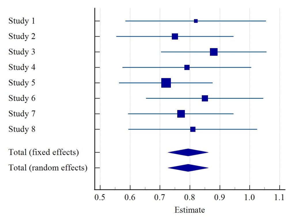
Components
Squares
Represent study estimates.
Larger squares indicate larger study weight.
Horizontal Lines
Represent 95% Confidence Intervals.
Shorter lines indicate greater precision.
Diamond
Represents pooled effect estimate.
Diamond width represents pooled 95% CI.
Study Results Interpretation
Individual Studies
| Study | Estimate | 95% CI | Weight (%) |
|---|---|---|---|
| Study 1 | 0.820 | 0.585–1.055 | 8.29 |
| Study 2 | 0.750 | 0.554–0.946 | 11.93 |
| Study 3 | 0.880 | 0.704–1.056 | 14.73 |
| Study 4 | 0.790 | 0.574–1.006 | 9.86 |
| Study 5 | 0.720 | 0.563–0.877 | 18.65 |
| Study 6 | 0.850 | 0.654–1.046 | 11.93 |
| Study 7 | 0.770 | 0.594–0.946 | 14.73 |
| Study 8 | 0.810 | 0.594–1.026 | 9.86 |
Study 5 contributes the highest weight because it has the smallest standard error.
Overall Meta-Analysis Result
Fixed Effect Model
| Statistic | Value |
|---|---|
| Pooled Estimate | 0.794 |
| Standard Error | 0.0345 |
| 95% CI | 0.726 – 0.862 |
| Z-value | 22.987 |
| P-value | <0.001 |
Random Effect Model
| Statistic | Value |
|---|---|
| Pooled Estimate | 0.794 |
| Standard Error | 0.0345 |
| 95% CI | 0.726 – 0.862 |
| Z-value | 22.987 |
| P-value | <0.001 |
Because heterogeneity is absent, fixed and random effects models produce identical results.
Interpretation of Overall Effect
The pooled estimate is:
0.794
95% Confidence Interval:
0.726 to 0.862
P-value:
<0.001
Interpretation
The combined effect estimate is statistically significant.
Since the confidence interval does not cross the null value and the P-value is less than 0.05, the overall effect is considered highly significant.
Heterogeneity Analysis
Meta-analysis must assess whether studies are consistent.
Cochran’s Q Test
| Statistic | Value |
|---|---|
| Q | 2.4164 |
| DF | 7 |
| P-value | 0.9333 |
Interpretation:
P > 0.05
No significant heterogeneity exists among studies.
I² Statistic
| Statistic | Value |
|---|---|
| I² | 0.00% |
| 95% CI | 0.00–7.06% |
Interpretation:
| I² Value | Interpretation |
|---|---|
| 0–25% | Low heterogeneity |
| 25–50% | Moderate heterogeneity |
| 50–75% | Substantial heterogeneity |
| >75% | High heterogeneity |
The observed I² value is 0%, indicating excellent consistency among studies.
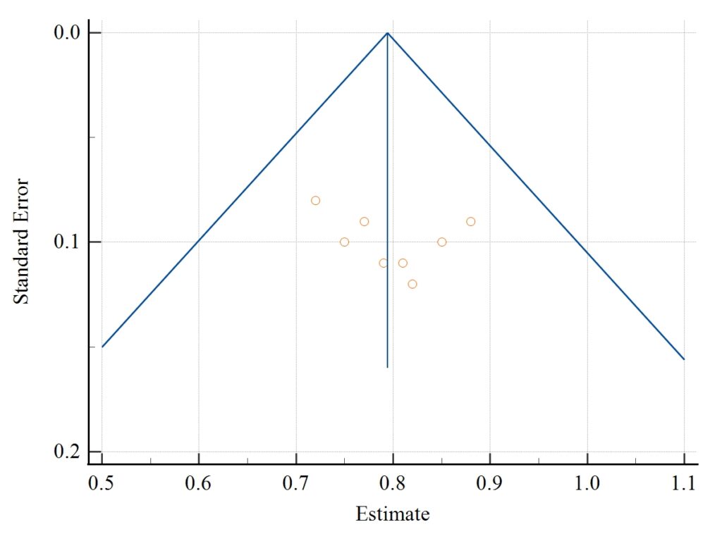
Funnel Plot Interpretation
The funnel plot is used to evaluate publication bias.
Expected Shape
A symmetric inverted funnel indicates:
- No publication bias
- Balanced distribution of studies
Current Funnel Plot
The plotted studies appear reasonably symmetric around the pooled estimate.
There is no obvious visual evidence of publication bias.
Publication Bias Tests
Egger’s Test
| Statistic | Value |
|---|---|
| Intercept | 1.6246 |
| 95% CI | -2.4810 to 5.7303 |
| P-value | 0.3703 |
Interpretation:
P > 0.05
No significant publication bias detected.
Begg’s Test
| Statistic | Value |
|---|---|
| Kendall Tau | 0.2646 |
| P-value | 0.3594 |
Interpretation:
P > 0.05
No evidence of publication bias.
Reporting Results in a Research Paper
Example Write-Up
“A meta-analysis using the Generic Inverse Variance Method was performed in MedCalc. The pooled estimate was 0.794 (95% CI: 0.726–0.862; P < 0.001), indicating a statistically significant overall effect. Heterogeneity among studies was negligible (Q = 2.4164, P = 0.9333; I² = 0.0%). Funnel plot assessment and publication bias tests showed no significant publication bias (Egger’s test P = 0.3703; Begg’s test P = 0.3594).”
Download Data File
To practice this analysis yourself, download the sample dataset used in this tutorial.
Download Sample Data (.xlsx):
Conclusion
The Generic Inverse Variance Method is one of the most flexible meta-analysis approaches available in MedCalc. It enables researchers to combine effect estimates and standard errors from multiple studies when raw data are unavailable. In this example, the pooled estimate was 0.794 with a highly significant P-value (<0.001), while heterogeneity was absent (I² = 0%). Both Egger’s and Begg’s tests confirmed the absence of publication bias. By understanding study weights, forest plots, funnel plots, heterogeneity statistics, and publication bias assessments, researchers can confidently perform and interpret meta-analyses using MedCalc. This method is particularly valuable for systematic reviews, observational studies, survival analyses, and evidence-based research where adjusted estimates are reported rather than raw outcomes.