Introduction
Data visualization is one of the most essential steps in biological research, ecological monitoring, agricultural experiments, and medical studies. Among all visualization techniques, the boxplot is widely used because it helps researchers quickly interpret the distribution, central tendency, and variability of data across multiple groups or treatments.
However, in modern biostatistics and data science, researchers prefer boxplots that show individual data points. This approach enhances transparency, avoids misinterpretation of summary-only visuals, and displays the underlying data distribution more clearly. Overlaying individual dots (jittered points) on a boxplot is especially useful when:
- The sample size is small
- Distribution patterns vary significantly
- You want to show both summary statistics and raw data
- The dataset belongs to biological or clinical experiments
In this article, you will learn how to create a boxplot with individual data points overlaid using R Studio and the ggplot2 package. This guide is fully structured for WordPress, provides step-by-step instructions, includes your script from the uploaded file, and explains where to insert images within the post for best SEO performance.
By the end, you will be able to produce a publication-ready figure suitable for theses, journal articles, laboratory reports, blog posts, and presentations.
📺 Video Tutorial: Boxplot with Individual Data Points in R
Watch the full step-by-step video tutorial on our YouTube channel StatisticsBio7:
Why Use Boxplots with Overlaid Points?
Standard boxplots show:
- Minimum
- 1st quartile (Q1)
- Median
- 3rd quartile (Q3)
- Maximum
But they do not display:
- How many observations exist
- Outlier density
- Clusters or patterns
- Skewness of data
- Biological variation across samples
Overlaying individual data points solves these problems.
This technique is now widely recommended in:
- Biostatistics
- Ecology
- Plant sciences
- Medical and clinical research
- Omics data analysis
- Agricultural field trials
It combines summary statistics (boxplot) with raw data transparency (jitter points), giving readers a more complete understanding.
Software Requirements
Before beginning, ensure you have:
- R (latest version)
- RStudio
- The R package ggplot2
- (Optional) The R package readxl if importing from Excel
Dataset Structure
To follow this tutorial, your data should have:
| Column | Description |
|---|---|
| Treatment | Grouping variable (factor) |
| Height_cm | Numerical measurement (continuous variable) |
Example biological datasets that match this structure:
- Plant height under different fertilizer treatments
- Animal weight across diet categories
- Enzyme activity across experimental conditions
- Growth rate under temperature or pH treatments
📥 Download Sample Dataset
You can download the example dataset used in this tutorial:
🔗 Click here to download the dataset (Excel)
Step-by-Step Guide to Create Boxplot with Individual Points
Step 1: Install and Load Required Packages
Copy and paste the below code into RStudio.
# Install ggplot2 (Run only once)
install.packages("ggplot2")

# Load ggplot2
library(ggplot2)
If you want to import Excel files, install and load readxl:
# Install readxl for importing Excel files
install.packages("readxl")

# Load readxl
library(readxl)
Step 2: Import Your Dataset
If your dataset is in Excel format:
plant_data <- read_excel("C:/Users/YourName/Documents/plant_data.xlsx")
If your dataset is a CSV file:
plant_data <- read.csv("plant_data.csv")
After loading:
head(plant_data)
This allows you to verify:
- Column names
- Data types
- Missing values
Step 3: Basic Boxplot with ggplot2
A classical boxplot without overlays:
ggplot(plant_data, aes(x = Treatment, y = Height_cm, fill = Treatment)) +
  geom_boxplot() +
  theme_minimal()
This plot shows only the distribution summary, not the raw observations.
Step 4: Add Individual Data Points (Jittered Points)
Your uploaded script script already includes a clean version of this advanced plot:
ggplot(plant_data, aes(x = Treatment, y = Height_cm, fill = Treatment)) +
  geom_boxplot(outlier.shape = NA, alpha = 0.5, width = 0.6) +
  geom_jitter(width = 0.15, size = 2, alpha = 0.8) +
  labs(title = "Plant Height under Different Treatments",
       x = "Treatment Type",
       y = "Plant Height (cm)") +
  theme_minimal(base_size = 14) +
  theme(legend.position = "none",
        plot.title = element_text(hjust = 0.5, face = "bold"))
Explanation of Each Line
Below is a full explanation for your WordPress readers.
1. ggplot(…, aes())
Defines the dataset and aesthetics:
- x-axis = Treatment (categorical)
- y-axis = Height_cm (numeric)
- fill = Treatment (group color)
2. geom_boxplot()
Draws the boxplot.
outlier.shape = NA
→ Removes outliers so the jittered points will represent them instead.
alpha = 0.5
→ Makes the box semi-transparent.
width = 0.6
→ Controls the width of the box.
3. geom_jitter()
Adds individual points with slight random horizontal movement.
width = 0.15
→ Prevents points from overlapping.
size = 2, alpha = 0.8
→ Controls dot appearance and transparency.
4. labs()
Adds title and axis labels.
5. theme_minimal(base_size = 14)
Clean, publication-ready theme.
6. legend.position = “none”
Since the fill color equals Treatment, a legend is unnecessary.
7. plot.title = element_text()
Centers and bolds the plot title.
Step 5: Save the Plot
To export the figure as a high-quality image:
ggsave("boxplot_points.png", width = 7, height = 5, dpi = 300)
Or save manually using:
RStudio → Plots Tab → Export → Save as Image
Additional Customizations (Advanced)
1. Change color palette
scale_fill_brewer(palette = "Set2")
2. Add mean points
stat_summary(fun = mean, geom = "point", size = 3, color = "black")
3. Draw a violin + boxplot + points combo
ggplot(plant_data, aes(Treatment, Height_cm, fill = Treatment)) +
  geom_violin(alpha = 0.4) +
  geom_boxplot(width = 0.15) +
  geom_jitter(width = 0.1)
4. Sort groups by median
plant_data$Treatment <- reorder(plant_data$Treatment, plant_data$Height_cm, median)
Applications in Biological Sciences
This visualization method is extremely useful in:
Plant Science
- Fertilizer trials
- Soil treatment experiments
- Drought vs normal conditions
Animal & Veterinary Science
- Feeding trials
- Weight comparison
- Behavioral variation studies
Medical & Clinical Research
- Biomarker levels
- Blood pressure, heart rate
- Pre-post intervention studies
Environmental Biology
- Pollution impact studies
- Species abundance variations
Because jittered boxplots display both statistical summary and variability, they are highly trustworthy, especially when sample sizes are small.
Common Mistakes and How to Avoid Them
Mistake 1: Not removing outlier symbols
Solution: Use outlier.shape = NA.
Mistake 2: Overplotting points
Solution: Use geom_jitter(width = 0.15).
Mistake 3: Missing factor conversion
Ensure the Treatment variable is:
plant_data$Treatment <- as.factor(plant_data$Treatment)
Mistake 4: Axis labels not meaningful
Always rename x and y axes clearly.
Full Final R Script for WordPress Readers
Below is the complete script (cleaned and ready for publication):
# Install required packages
install.packages("ggplot2")      # Run once
install.packages("readxl")       # Only if importing Excel

# Load libraries
library(ggplot2)
library(readxl)

# Import dataset (example path)
plant_data <- read_excel("C:/Users/YourName/Documents/plant_data.xlsx")

# Inspect dataset
head(plant_data)

# Create Boxplot with Individual Data Points Overlaid
ggplot(plant_data, aes(x = Treatment, y = Height_cm, fill = Treatment)) +
  geom_boxplot(outlier.shape = NA, alpha = 0.5, width = 0.6) +
  geom_jitter(width = 0.15, size = 2, alpha = 0.8) +
  labs(title = "Plant Height under Different Treatments",
       x = "Treatment Type",
       y = "Plant Height (cm)") +
  theme_minimal(base_size = 14) +
  theme(legend.position = "none",
        plot.title = element_text(hjust = 0.5, face = "bold"))

# Save output
ggsave("boxplot_points.png", width = 7, height = 5, dpi = 300)
Conclusion
Creating a boxplot with individual data points overlaid in R Studio is one of the most effective ways to visualize experimental results in the biological sciences. It provides a transparent, visually appealing, and scientifically robust method to display both summary statistics and raw observations.
Using ggplot2, researchers can easily customize their plots, enhance clarity, and generate publication-ready figures for theses, manuscripts, posters, or online articles. The method demonstrated in this tutorial is widely accepted in top scientific journals and is now considered a best practice in biostatistical reporting.