Introduction
Pearson correlation in biostatistics is one of the most commonly used statistical methods for studying the relationship between two quantitative variables. It helps researchers determine whether changes in one variable are associated with changes in another variable and describes both the direction and strength of a linear relationship.
In biological and medical research, Pearson correlation can be used to investigate relationships such as age and blood pressure, body weight and blood glucose, drug concentration and response, or laboratory measurements between two experimental variables.
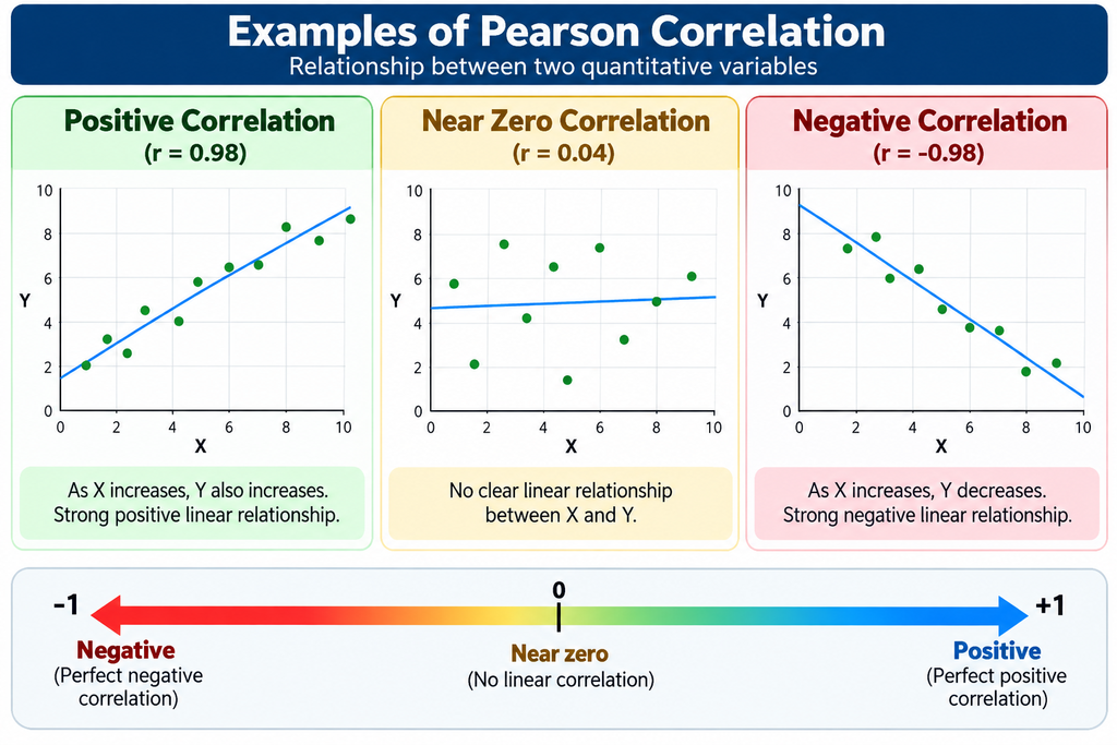
The Pearson correlation coefficient is represented by r and ranges from −1 to +1. A value close to +1 indicates a strong positive linear relationship, while a value close to −1 indicates a strong negative linear relationship. A value near 0 indicates little or no linear association.
Importantly, correlation describes an association between variables; it does not by itself establish causation.
What Is Pearson Correlation?
Pearson correlation is a statistical technique used to measure the strength and direction of the linear relationship between two continuous quantitative variables.
The Pearson correlation coefficient is calculated as:
Where:
- r = Pearson correlation coefficient
- X = observations of the first variable
- Y = observations of the second variable
- X̄ = mean of X
- Ȳ = mean of Y
The coefficient always lies between −1 and +1.
General interpretation
| Pearson r | General interpretation |
|---|---|
| +1.00 | Perfect positive linear correlation |
| +0.70 to +0.99 | Strong positive correlation |
| +0.40 to +0.69 | Moderate positive correlation |
| +0.10 to +0.39 | Weak positive correlation |
| 0.00 | No linear correlation |
| −0.10 to −0.39 | Weak negative correlation |
| −0.40 to −0.69 | Moderate negative correlation |
| −0.70 to −0.99 | Strong negative correlation |
| −1.00 | Perfect negative linear correlation |
These ranges are general descriptive guidelines, not universal statistical rules. Interpretation should also consider the scientific context and sample size.
Concept of Pearson Correlation
Pearson correlation examines whether two variables tend to change together in a linear pattern.
For example, suppose a researcher measures the body weight and systolic blood pressure of several participants. If participants with greater body weight generally have higher systolic blood pressure, the relationship may be positive.
Conversely, if increasing one variable is generally associated with decreasing another variable, the relationship is negative.
Pearson Correlation in Biostatistics: Step-by-Step
Step 1: Identify the two variables
Select two quantitative variables that you want to compare.
For example:
- X = Body weight (kg)
- Y = Systolic blood pressure (mmHg)
Both variables should be measured for the same individuals or experimental units.
Step 2: Organize the data
Arrange the observations in two corresponding columns.
| Participant | Body Weight (kg) | Systolic BP (mmHg) |
|---|---|---|
| 1 | 50 | 110 |
| 2 | 55 | 114 |
| 3 | 60 | 118 |
| 4 | 65 | 124 |
| 5 | 70 | 128 |
| 6 | 75 | 132 |
| 7 | 80 | 138 |
| 8 | 85 | 142 |
This dataset shows a generally increasing pattern.
Step 3: Examine the scatterplot
Before calculating Pearson’s correlation, create a scatterplot.
A scatterplot can reveal:
- Positive or negative direction
- Approximate strength of association
- Possible outliers
- Whether the relationship appears linear
- Possible unusual patterns
Step 4: Calculate the correlation coefficient
Statistical software calculates the Pearson correlation coefficient using the observed X and Y values.
The result might be, for example:
r = 0.99
This would indicate a very strong positive linear association in this illustrative dataset.
Step 5: Test statistical significance
Researchers commonly test:
- Null hypothesis (H₀): There is no linear correlation in the population.
- Alternative hypothesis (H₁): There is a linear correlation in the population.
A p-value is usually reported along with the correlation coefficient.
For example:
r = 0.99, p < 0.001
This indicates strong evidence against the null hypothesis of zero population linear correlation, under the assumptions of the test.
Step 6: Interpret the result in context
The statistical result should be translated into a biological or clinical interpretation.
For example:
There was a strong positive linear association between body weight and systolic blood pressure in the study sample.
The wording should avoid claiming that increased body weight caused increased blood pressure unless a suitable causal study design and analysis support such a conclusion.
Example of Pearson Correlation
Consider a study investigating the relationship between body weight and systolic blood pressure.
Suppose the analysis produces:
Pearson correlation: r = 0.82
p-value: < 0.001
The coefficient of 0.82 indicates a strong positive linear association. The p-value provides evidence that the observed association is unlikely to be explained by sampling variation alone under the null hypothesis of zero population correlation.
A suitable report could be:
Pearson correlation analysis demonstrated a strong positive association between body weight and systolic blood pressure (r = 0.82, p < 0.001).
Important Assumptions
Before using Pearson correlation, researchers should consider several assumptions.
1. Quantitative variables
The two variables should generally be continuous or approximately continuous quantitative measurements.
2. Linear relationship
Pearson correlation measures linear association. A strong curved relationship can produce a relatively small Pearson correlation.
3. Independence
Observations should generally be independent of one another. Repeated measurements from the same participant require methods that account for within-subject dependence.
4. Outliers
Extreme observations can substantially influence Pearson’s correlation coefficient. Scatterplots should therefore be examined before interpreting the result.
5. Distributional considerations
For significance testing and confidence intervals, additional assumptions concerning the joint distribution of the variables are relevant. In small samples, severe departures from assumptions can affect inference.
When assumptions are inappropriate, Spearman’s rank correlation may be considered, depending on the research question and data characteristics.
Pearson Correlation vs. Spearman Correlation
| Feature | Pearson Correlation | Spearman Correlation |
|---|---|---|
| Main relationship | Linear | Monotonic |
| Data | Quantitative | Ordinal or quantitative |
| Uses actual values | Yes | Uses ranks |
| Sensitive to outliers | Relatively sensitive | Generally less sensitive |
| Distribution assumptions | More assumptions for inference | Fewer distributional assumptions |
| Common application | Linear association | Ranked/monotonic association |
The choice between Pearson and Spearman should be based on the research question, measurement scale, data pattern, and assumptions rather than simply choosing one because its p-value is more favorable.
Applications in Biostatistics
Pearson correlation is widely applicable in biomedical and biological research.
Clinical research
Researchers can investigate relationships between:
- Age and blood pressure
- Weight and cholesterol
- Biomarker concentration and disease measurements
- Laboratory measurements and clinical variables
Epidemiology
Correlation can be used to explore relationships between quantitative population-level measurements, such as environmental exposure and disease-related measurements.
Laboratory research
Researchers may compare two laboratory measurement techniques or examine associations between biochemical parameters.
Biological research
Pearson correlation can help investigate relationships between variables such as growth measurements, environmental factors, physiological parameters, and experimental responses.
However, the study design and measurement structure should always be considered before applying correlation analysis.
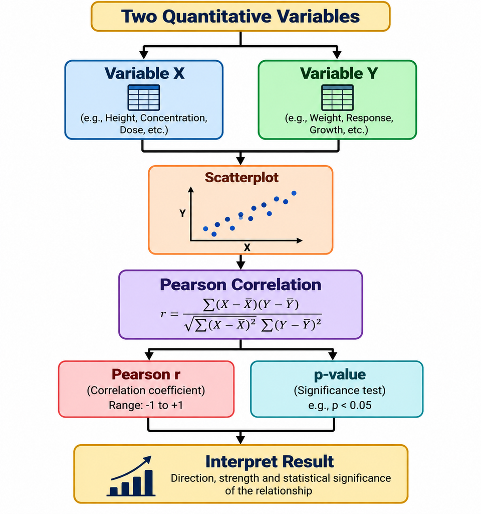
Pearson Correlation Concept
A simple conceptual representation can be shown as:
Advantages of Pearson Correlation
Pearson correlation has several advantages:
- It is easy to calculate and interpret.
- It provides both direction and strength of linear association.
- It is widely implemented in statistical software.
- It is useful for exploratory biomedical research.
- It can be presented together with scatterplots and regression analyses.
- It provides a standardized coefficient ranging from −1 to +1.
Limitations of Pearson Correlation
Despite its usefulness, Pearson correlation has important limitations.
A correlation coefficient does not establish causation. Two variables may be correlated because of a third variable or because of other features of the study design.
Pearson correlation also focuses specifically on linear association. Therefore, a nonlinear relationship may not be adequately represented by the coefficient.
Outliers can strongly affect the calculated value, so researchers should inspect the data visually before drawing conclusions.
Finally, statistical significance does not necessarily mean that an association is biologically or clinically important. The magnitude of the effect, confidence interval, study design, and scientific context should also be considered.
Conclusion
Pearson correlation in biostatistics is an important statistical method for measuring the strength and direction of a linear relationship between two quantitative variables. The Pearson correlation coefficient ranges from −1 to +1, with the sign indicating the direction and the magnitude describing the strength of the linear association.
A proper correlation analysis should involve more than simply reporting a p-value. Researchers should inspect scatterplots, consider assumptions and outliers, report the correlation coefficient with appropriate statistical inference, and interpret the findings within the biological or clinical context.
When used appropriately, Pearson correlation provides a simple and valuable approach for exploring relationships in biostatistics, clinical research, laboratory studies, epidemiology, and biological research.