Introduction
Meta-analysis is a powerful statistical technique used to combine results from multiple independent studies and generate a single overall estimate. In evidence-based medicine, meta-analysis improves statistical power and provides more reliable conclusions than individual studies.
One commonly used effect size measure for binary outcomes is the Risk Difference (RD). Risk Difference quantifies the absolute difference in event rates between treatment and control groups.
In this tutorial, you will learn how to perform Meta-Analysis Risk Difference in MedCalc, understand all software options, interpret forest plots and funnel plots, assess heterogeneity, evaluate publication bias, and report findings correctly.
The example used in this article is based on a biomedical dataset comparing treatment and control groups for a clinical outcome. The MedCalc output showed a pooled Risk Difference of -0.145, indicating a significant reduction in risk in the treatment group.
What is Risk Difference?
Risk Difference (RD) is the absolute difference in event probabilities between two groups.
Formula
Risk Difference = Treatment Risk − Control Risk
Where:
- Treatment Risk = Positive outcomes / Total treatment subjects
- Control Risk = Positive outcomes / Total control subjects
Interpretation
| Risk Difference | Meaning |
|---|---|
| RD = 0 | No difference |
| RD > 0 | Higher risk in treatment group |
| RD < 0 | Lower risk in treatment group |
| RD = -0.10 | 10% absolute risk reduction |
Risk Difference is particularly useful in clinical research because it provides an absolute measure of benefit rather than a relative measure.
Why Use Meta-Analysis Risk Difference?
Researchers use Risk Difference when:
- Outcomes are binary (Yes/No)
- Comparing treatment versus control groups
- Assessing intervention effectiveness
- Performing systematic reviews
- Calculating absolute treatment benefit
Examples include:
- Disease occurrence
- Mortality
- Recovery rate
- Vaccine effectiveness
- Adverse event incidence
Example Biomedical Dataset
The following dataset was used for the analysis:
| Study | Treat Positive | Treat Total | Control Positive | Control Total |
|---|---|---|---|---|
| Study 1 | 30 | 200 | 60 | 200 |
| Study 2 | 28 | 180 | 52 | 180 |
| Study 3 | 40 | 250 | 78 | 250 |
| Study 4 | 35 | 220 | 65 | 220 |
| Study 5 | 48 | 300 | 92 | 300 |
| Study 6 | 42 | 280 | 85 | 280 |
| Study 7 | 36 | 240 | 70 | 240 |
| Study 8 | 39 | 260 | 75 | 260 |
This dataset evaluates whether a treatment reduces the occurrence of a specific clinical outcome compared with a control group.
Download Dataset
📥 Meta-Analysis Risk Difference Dataset.xlsx
Step-by-Step Analysis in MedCalc
Step 1
Open MedCalc.
Navigate to:
Statistics → Meta-analysis → Risk Difference
Step 2
Select the following variables.
Studies
Study
Intervention Groups
Total Number of Cases
Treat_Total
Number with Positive Outcome
Treat_Positive
Control Groups
Total Number of Cases
Control_Total
Number with Positive Outcome
Control_Positive
Step 3
Configure analysis options.
Options Explanation
Forest Plot
Displays effect size and confidence intervals for each study.
Purpose:
- Compare studies visually
- Display pooled effect
- Evaluate consistency
Recommended: ✔ Yes
Marker Size Relative to Study Weight
Larger studies receive larger squares.
Benefits:
- Shows contribution of each study
- Visualizes weighting scheme
Recommended: ✔ Yes
Fixed Effect Model Weights
Assumes all studies estimate the same true effect.
Use when:
- Heterogeneity is negligible
- I² is very low
Recommended for this dataset because I² = 0%.
Random Effect Model Weights
Assumes studies may estimate different true effects.
Use when:
- Studies differ substantially
- Heterogeneity exists
Recommended in most biomedical meta-analyses.
Plot Pooled Effect – Fixed Effects Model
Displays pooled estimate using fixed-effect assumptions.
Plot Pooled Effect – Random Effects Model
Displays pooled estimate using random-effects assumptions.
Recommended: ✔ Yes
Diamonds for Pooled Effects
Displays pooled effect as a diamond in the forest plot.
Diamond width represents the confidence interval.
Recommended: ✔ Yes
Funnel Plot
Used to evaluate publication bias.
Recommended: ✔ Yes
Manual Risk Difference Calculation Example
Using Study 1:
Treatment Risk:
30 / 200 = 0.15
Control Risk:
60 / 200 = 0.30
Risk Difference:
RD = 0.15 − 0.30
RD = -0.15
Interpretation:
Treatment reduced risk by 15 percentage points.
Results Summary
According to the MedCalc output:
| Model | Risk Difference | 95% CI | P-value |
|---|---|---|---|
| Fixed Effect | -0.145 | -0.171 to -0.119 | <0.001 |
| Random Effect | -0.145 | -0.171 to -0.118 | <0.001 |
The pooled estimate shows a statistically significant reduction in risk in the treatment group.
Individual Study Results
| Study | Risk Difference |
|---|---|
| Study 1 | -0.150 |
| Study 2 | -0.133 |
| Study 3 | -0.152 |
| Study 4 | -0.136 |
| Study 5 | -0.147 |
| Study 6 | -0.154 |
| Study 7 | -0.142 |
| Study 8 | -0.138 |
All studies consistently favored the treatment group.
Forest Plot Interpretation
The forest plot summarizes all studies visually.
Components
Squares
Represent effect estimates from individual studies.
Larger squares indicate greater study weight.
Horizontal Lines
Represent 95% confidence intervals.
Diamond
Represents the pooled effect estimate.
Interpretation of This Forest Plot
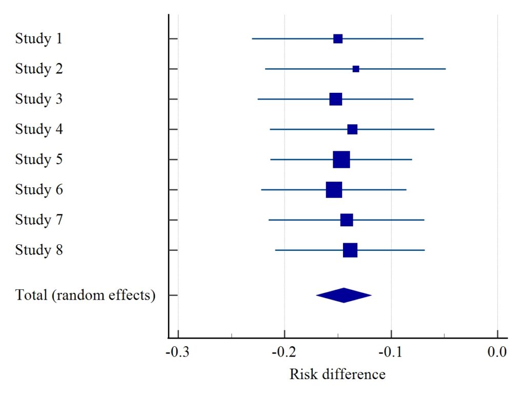
The pooled random-effects estimate is:
RD = -0.145
95% CI:
-0.171 to -0.118
Because the confidence interval does not cross zero, the result is statistically significant.
Conclusion from Forest Plot
The treatment significantly reduced the clinical outcome risk by approximately 14.5%.
Heterogeneity Analysis
Heterogeneity measures variability among studies.
MedCalc reported:
| Statistic | Value |
|---|---|
| Q | 0.2738 |
| DF | 7 |
| P-value | 0.9999 |
| I² | 0.00% |
Interpretation
I² = 0%
Meaning:
- No heterogeneity
- Excellent agreement among studies
- Results are highly consistent
Because heterogeneity is absent, fixed-effect and random-effect results are almost identical.
Funnel Plot Interpretation
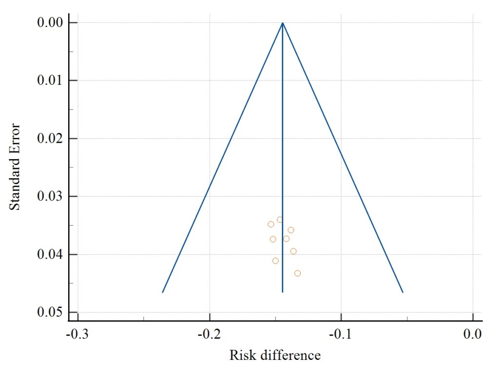
The funnel plot assesses publication bias.
A symmetrical funnel indicates:
- Low publication bias
- Balanced study distribution
The funnel plot generated from this analysis appears reasonably symmetrical.
Publication Bias Results
Egger’s Test
| Statistic | Value |
|---|---|
| Intercept | 1.1112 |
| P-value | 0.2532 |
Begg’s Test
| Statistic | Value |
|---|---|
| Kendall Tau | 0.3571 |
| P-value | 0.2160 |
Interpretation
Both P-values are greater than 0.05.
Therefore:
✔ No significant publication bias detected.
The included studies appear balanced and reliable.
How to Report Results in a Research Paper
Example:
A meta-analysis of eight studies showed a significant reduction in risk among treated participants compared with controls (RD = -0.145, 95% CI: -0.171 to -0.118, P < 0.001). No significant heterogeneity was observed (I² = 0.0%), and publication bias was not detected using Egger’s and Begg’s tests.
Advantages of Risk Difference
- Easy clinical interpretation
- Measures absolute benefit
- Useful for treatment recommendations
- Supports Number Needed to Treat calculations
- Widely used in evidence-based medicine
Conclusion
Meta-Analysis Risk Difference is a valuable method for evaluating treatment effectiveness using binary outcome data. In this MedCalc example, the pooled Risk Difference was -0.145, indicating that the treatment reduced risk by approximately 14.5% compared with the control group. The forest plot demonstrated consistent effects across all studies, while heterogeneity analysis showed I² = 0%, indicating excellent agreement among studies. Publication bias assessments using Egger’s and Begg’s tests were non-significant, supporting the reliability of the findings.
This workflow provides researchers with a clear and practical approach for conducting Risk Difference meta-analysis and interpreting results confidently in biomedical research.