Introduction
Time series regression is a powerful statistical technique widely used in environmental health, epidemiology, economics, and social sciences to understand how an outcome changes over time in relation to one or more explanatory variables. In public health research, time series regression is especially useful for studying short-term associations between environmental exposures—such as air pollution or temperature—and health outcomes like asthma, cardiovascular diseases, or hospital admissions.
What Is Time Series Regression?
Time series regression is a regression model in which observations are ordered in time. Unlike simple cross-sectional data, time series data may show trends, seasonality, and autocorrelation. In environmental health studies, time series regression helps quantify how short-term changes in pollution or weather are associated with health outcomes.
In this example:
- Outcome variable: Asthma cases (monthly counts)
- Predictor variables: PM2.5, lagged PM2.5, temperature
- Additional variable: Intervention (policy or environmental change indicator)
Description of the Dataset
The dataset used in this study consists of monthly observations from February to December 2020. Each row represents one month.
Table 1. Description of Variables Used in Time Series Regression
| Variable Name | Description |
|---|---|
| Month | Monthly time variable (Date format) |
| Asthma | Number of reported asthma cases |
| PM2.5 | Monthly average PM2.5 concentration (µg/m³) |
| Lag_PM2.5 | Previous month’s PM2.5 concentration |
| Temp | Monthly average temperature (°C) |
| Intervention | Indicator variable (0 = before, 1 = after intervention) |
Download Dataset
Step-by-Step: How to Enter and Run the Script in R Studio
Step 1: Open R Studio
- Launch R Studio on your computer
- Open a new script file: File → New File → R Script
Step 2: Install and Load Required Packages
If the packages are not installed, run the following once:
install.packages(c("ggplot2", "dplyr", "lubridate", "gridExtra"))
Then load the libraries:
library(ggplot2)
library(dplyr)
library(lubridate)
library(gridExtra)
Step 3: Create the Dataset
Copy and paste the dataset creation code into your script. This step defines the time variable and all predictors used in the model.
Step 4: Fit the Time Series Regression Model
Use the lm() function to fit the regression model:
model <- lm(Asthma ~ PM2.5 + Lag_PM2.5 + Temp + Intervention, data = data)
summary(model)
This command estimates the association between asthma cases and the predictors.
Step 5: Visualize the Time Series Data
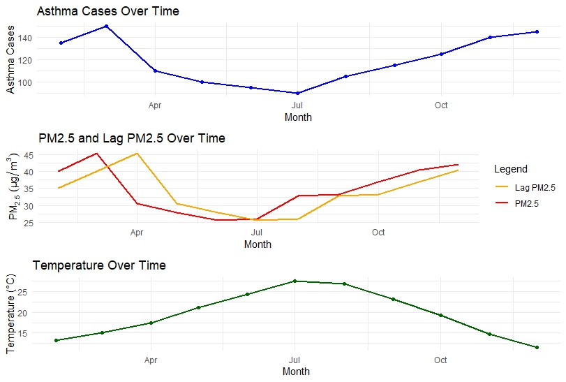
Three plots are generated:
- Asthma cases over time
- PM2.5 and lagged PM2.5 over time
- Temperature over time
These plots help visually inspect trends and seasonal patterns.
Time Series Plots: Visual Interpretation
Asthma Cases Over Time
The asthma time series shows a decline from early summer, followed by a steady increase toward the end of the year. This pattern may reflect seasonal effects or changes in environmental exposure.
PM2.5 and Lagged PM2.5
PM2.5 levels decrease during mid-year and increase again toward winter. The lagged PM2.5 curve closely follows the original series, indicating temporal persistence of air pollution.
Temperature Over Time
Temperature peaks during mid-year and declines toward the end of the year, showing a clear seasonal trend.
These visual patterns justify the use of a time series regression framework.
Regression Results and Interpretation
Model Summary
The fitted time series regression model explains a very high proportion of variability in asthma cases.
- Multiple R-squared: 0.9929
- Adjusted R-squared: 0.9881
- Overall model p-value: < 0.001
This indicates an excellent model fit.
Interpretation of Coefficients
- PM2.5: A statistically significant positive association with asthma cases. An increase in PM2.5 is associated with an increase in asthma cases, highlighting the strong impact of air pollution.
- Lagged PM2.5: The effect is positive but not statistically significant, suggesting that immediate exposure has a stronger effect than delayed exposure in this dataset.
- Temperature: Shows a negative association with asthma cases. Higher temperatures are linked with fewer asthma cases, possibly due to seasonal respiratory patterns.
- Intervention: The coefficient is positive but not statistically significant, indicating no strong evidence of an intervention effect during the study period.
Why Use Lag Variables in Time Series Regression?
Lag variables capture delayed effects of exposure. In environmental epidemiology, pollutants may not cause immediate health effects; symptoms can appear days or weeks later. Including lagged PM2.5 helps assess whether previous exposure influences current asthma cases.
Practical Applications
Time series regression models like this are widely used to:
- Assess health effects of air pollution
- Evaluate environmental policies
- Study climate–health relationships
- Support public health decision-making
Conclusion
This article demonstrated how to perform Time Series Regression in R Studio using environmental health data. By combining asthma case counts with PM2.5, lagged PM2.5, temperature, and an intervention variable, we illustrated how regression modeling and visualization can uncover meaningful temporal relationships.
The results emphasize the strong association between air pollution and asthma while highlighting the importance of temperature and temporal structure in health data. With clear plots, well-defined variables, and step-by-step R code, this approach is highly suitable for teaching, research, and applied public health analysis.
Time series regression in R Studio is a valuable skill for anyone working with longitudinal data, and this example provides a solid foundation for more advanced analyses such as generalized additive models or distributed lag models.