Introduction
In statistics, the concept of normally distributed data is fundamental for understanding many analytical methods and research outcomes. Normally distributed data, often referred to as a Gaussian distribution, describes a dataset where most values cluster around the mean, and the frequency of values decreases symmetrically as you move away from the mean. This distribution is widely observed in natural phenomena, biological measurements, psychological testing, and social sciences. Understanding whether data are normally distributed is critical for selecting the right statistical tests, interpreting results accurately, and drawing valid conclusions.
Many students and researchers encounter terms like “assume normality” or “data must be normally distributed” in textbooks and research papers. These statements can be confusing without a clear understanding of the concept. This article explains normally distributed data, its properties, examples, and applications in research and statistics.
Meaning of Normally Distributed Data
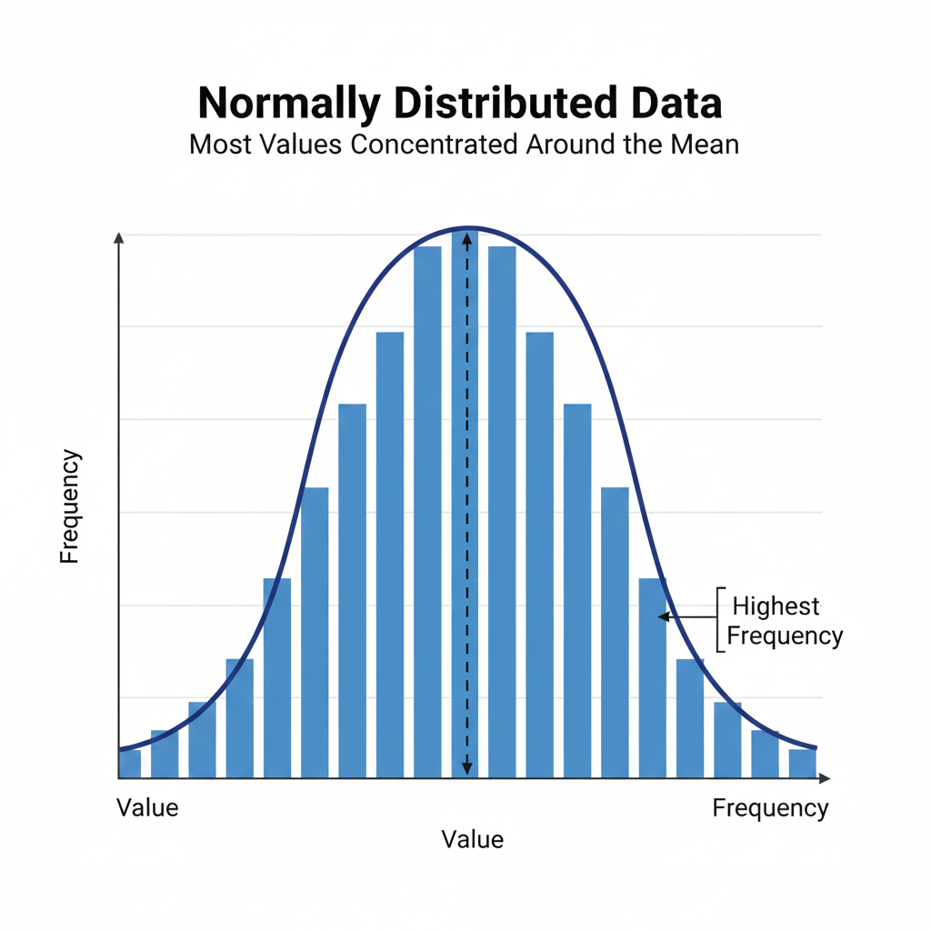
Normally distributed data is characterized by a bell-shaped curve where most observations are close to the mean, and fewer observations occur at the extremes. The mean, median, and mode of a perfectly normal distribution are equal and located at the center of the curve. The distribution is symmetric, meaning the left and right sides of the curve are mirror images.
This type of distribution allows statisticians to predict the probability of certain outcomes, calculate confidence intervals, and apply parametric tests, which are more powerful than non-parametric alternatives when the normality assumption holds. Recognizing normal distribution in your dataset ensures accurate statistical modeling and reliable results.
Properties of Normally Distributed Data
Normally distributed data has several important properties that make it essential in statistical analysis. First, the distribution is symmetric about the mean, and the mean, median, and mode are identical. Second, the total area under the curve equals one, representing the probability of all possible outcomes. Third, approximately 68% of the data falls within one standard deviation of the mean, 95% within two standard deviations, and 99.7% within three standard deviations—a principle known as the empirical rule.
These properties allow researchers to calculate probabilities, identify outliers, and compare datasets effectively. For example, if a student’s test score falls more than two standard deviations above the mean, it can be interpreted as an exceptional performance in the context of normally distributed scores.
Examples of Normally Distributed Data
Many real-world phenomena follow a normal distribution. In biology, measurements like human height, blood pressure, or weight often approximate a normal distribution. In psychology, intelligence scores such as IQ are designed to follow a normal distribution. In economics and social sciences, certain financial metrics, reaction times, or survey responses may exhibit normality.
For instance, measuring the blood pressure of 100 adults may result in a distribution where most individuals have readings around the mean, while very low or very high readings are rare. Recognizing this pattern helps in applying appropriate statistical tests and interpreting health-related trends accurately.
Checking for Normality
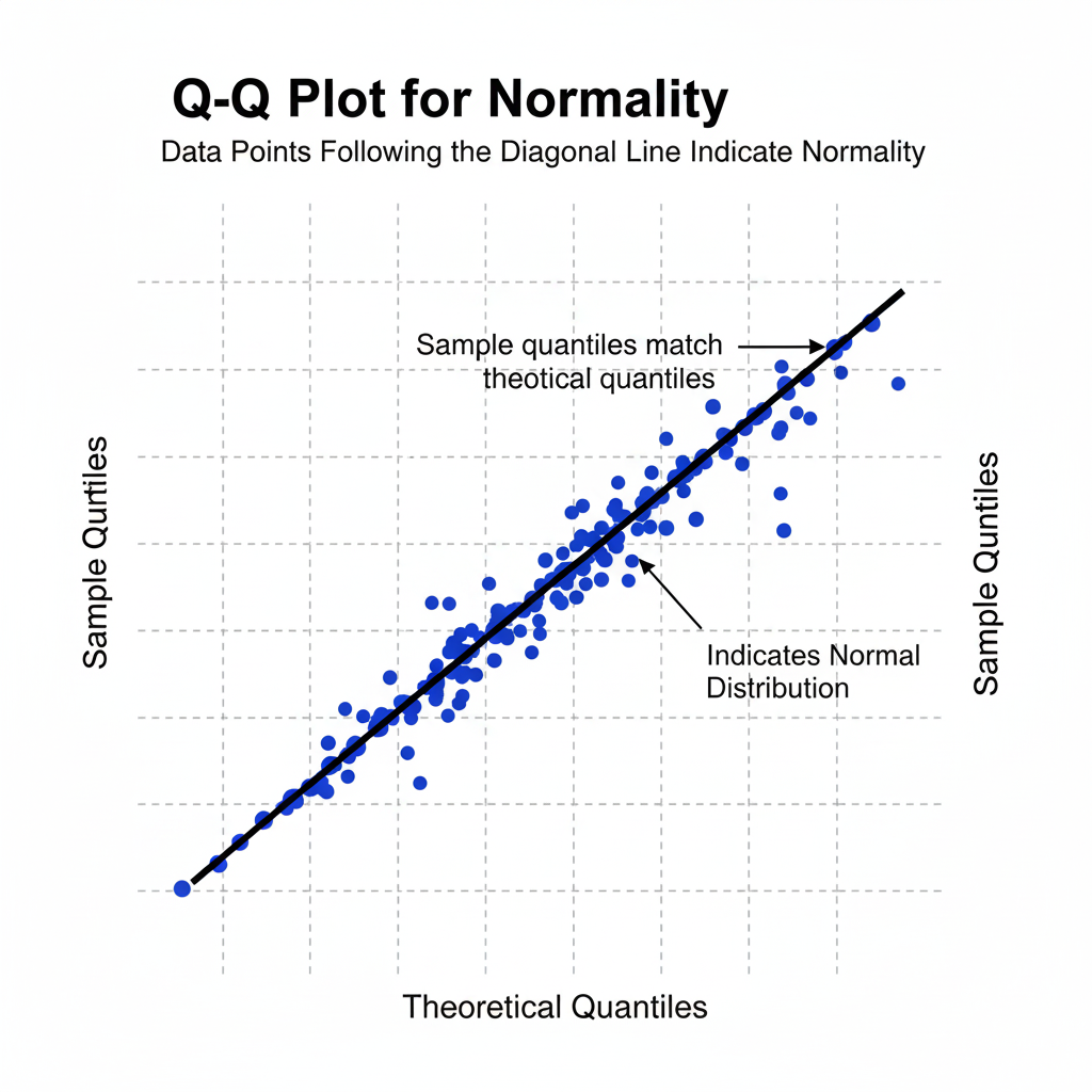
Before applying many statistical tests, it is important to determine whether the data are normally distributed. There are several methods to check normality. Graphical methods include histograms, boxplots, and Q-Q plots, which visually indicate whether data approximate a bell-shaped curve. Statistical tests such as the Shapiro-Wilk test, Kolmogorov-Smirnov test, and Anderson-Darling test provide numerical evidence of normality.
For example, in a Shapiro-Wilk test, a p-value greater than 0.05 suggests that the data do not significantly deviate from normality, allowing the use of parametric tests. If data fail normality tests, researchers may need to apply data transformation or use non-parametric tests that do not assume normality.
Importance in Statistical Analysis
The concept of normally distributed data is essential because many parametric tests assume normality. Tests like the t-test, paired sample t-test, ANOVA, and linear regression rely on the assumption that data or residuals are normally distributed. When this assumption holds, these tests are more powerful and yield more reliable results.
In practice, assuming normality simplifies probability calculations and confidence interval estimation. It allows researchers to predict outcomes with statistical certainty and supports hypothesis testing. Even when data are not perfectly normal, many parametric tests are robust enough to tolerate minor deviations, particularly with large sample sizes.
Applications in Research
Normally distributed data is applied across multiple fields. In medicine, researchers analyze clinical measurements, such as cholesterol levels or glucose readings, assuming approximate normality. In psychology, standardized tests rely on normal distribution to interpret scores relative to population averages. In economics, analysts model income or expenditure patterns, assuming data are normally distributed for forecasting and hypothesis testing.
For example, in a clinical trial measuring the effect of a new drug, researchers assume normally distributed blood pressure readings to calculate the mean difference, standard deviation, and confidence intervals. Understanding normal distribution ensures accurate statistical interpretation and valid conclusions.
Limitations and Misconceptions
While normal distribution is powerful, it is not universal. Many datasets, such as income, disease incidence, or reaction times, may be skewed or follow other distributions. Blindly assuming normality can lead to incorrect results. Researchers must always verify normality before applying parametric tests.
Another misconception is that all datasets must be perfectly normal. In reality, many statistical methods are robust to minor deviations from normality, especially with large sample sizes. The key is to check for severe skewness or outliers that can distort results and to apply transformations or non-parametric tests when necessary.
Visual Representation
A normal distribution is typically represented as a bell-shaped curve with the peak at the mean. The tails extend infinitely in both directions but never touch the x-axis. Visualizations help learners and researchers understand symmetry, the empirical rule, and the significance of standard deviations.
Graphical checks such as histograms or Q-Q plots are invaluable for confirming whether data can be assumed normal before proceeding with advanced statistical analysis.
Conclusion
Understanding normally distributed data is fundamental for accurate statistical analysis. Recognizing the bell-shaped pattern, checking normality, and applying appropriate tests are essential skills for students, researchers, and scientists. Normally distributed data underpins many parametric methods and allows researchers to make precise predictions, calculate probabilities, and interpret outcomes reliably.
Even when data are not perfectly normal, understanding the concept helps in choosing the correct transformations or non-parametric alternatives. Mastery of this concept strengthens research analysis, supports evidence-based conclusions, and ensures clarity and reliability in statistical reporting.